Introduction

The RMS Titanic was a British ship-liner that sunk due to a collision with an iceberg on April 15 1912. The total number of casualties was approximated to be 1,500. It was one of the largest passenger liners of its time, and the wreckage made global news. It was also made famous by the film appropriately named Titanic starring a young Leonardo Di Caprio, and directed by James Cameron.

Data

The source of this data comes from a competition on Kaggle. We are asked to successfully predict the survival status of passengers by numerous variables such as the passenger class, sex, age, etc. The survival status is our target variable, and is (obviously) binary, the task at hand is to predict the target variable by successfully constructing a machine learning model with a high degree of accuracy. Lets start by examining the structure of our data first, doing some exploratory analysis afterwards, and subsequently building our model.

titanic_train <- read.csv(file = '../../../train.csv', stringsAsFactors = FALSE, header = TRUE)
head(titanic_train)

##   PassengerId Survived Pclass
## 1           1        0      3
## 2           2        1      1
## 3           3        1      3
## 4           4        1      1
## 5           5        0      3
## 6           6        0      3
##                                                  Name    Sex Age SibSp
## 1                             Braund, Mr. Owen Harris   male  22     1
## 2 Cumings, Mrs. John Bradley (Florence Briggs Thayer) female  38     1
## 3                              Heikkinen, Miss. Laina female  26     0
## 4        Futrelle, Mrs. Jacques Heath (Lily May Peel) female  35     1
## 5                            Allen, Mr. William Henry   male  35     0
## 6                                    Moran, Mr. James   male  NA     0
##   Parch           Ticket    Fare Cabin Embarked
## 1     0        A/5 21171  7.2500              S
## 2     0         PC 17599 71.2833   C85        C
## 3     0 STON/O2. 3101282  7.9250              S
## 4     0           113803 53.1000  C123        S
## 5     0           373450  8.0500              S
## 6     0           330877  8.4583              Q

The “PassengerId” is a unique identifier and is not pertinent to our analysis or model. It’s also doubtful that we can gain any insight about the target variable from the passenger name, or ticket number. One could assume that the most relevant insight the ticket number would give us is Passenger Class, Fare Cost, and the port of embarkation (which is already given, conviniently).Therefore, we will eliminate these columns from our data set

train<- titanic_train[,-c(1,4,9,11)]
head(train)

##   Survived Pclass    Sex Age SibSp Parch    Fare Embarked
## 1        0      3   male  22     1     0  7.2500        S
## 2        1      1 female  38     1     0 71.2833        C
## 3        1      3 female  26     0     0  7.9250        S
## 4        1      1 female  35     1     0 53.1000        S
## 5        0      3   male  35     0     0  8.0500        S
## 6        0      3   male  NA     0     0  8.4583        Q

Unfortunately, we see that there are 177 missing values for the age variable. Hastily, we will just omit these observations. We’ll impute the values later.

train <- train[complete.cases(train),]

We plan on building a machine learning classifier. My gut instinct tells me to check and see if any socio-economic variables (sex, age, or number of children, fare cost, etc), correspond to a higher predisposition for death. Lets begin with ticket fare.

Exploratory Analysis

library(ggplot2)
train$Survived <- as.factor(train$Survived)
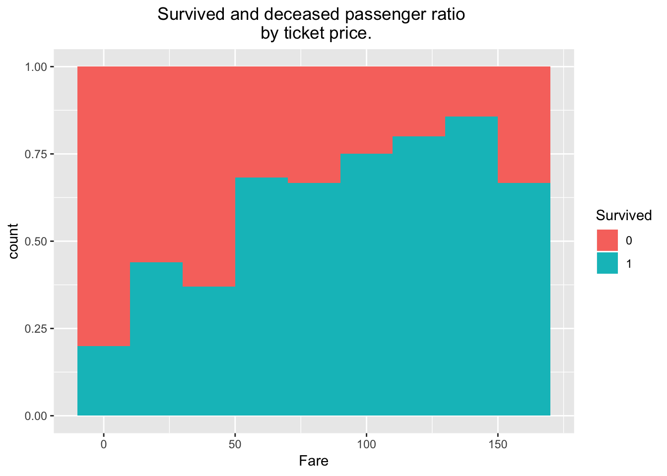
ggplot(train[train$Fare < 200,], aes(x = Fare, fill = Survived)) + geom_histogram(position = "fill", binwidth = 20) + ggtitle("Survived and deceased passenger ratio \n by ticket price.") + theme(plot.title = element_text(hjust = 0.5))

This is remarkable. If you were a passenger on the Titanic, you had a high chance of survival if you bought your ticket at the $100- $150 range. I must also note that this plot only accounts for tickets under $200, due to irregularly higher ticket purchase numbers being low, and skewing the plot leftwards. Nevertheless ticket sales above $200 only make up for less than 3% of total purchases.

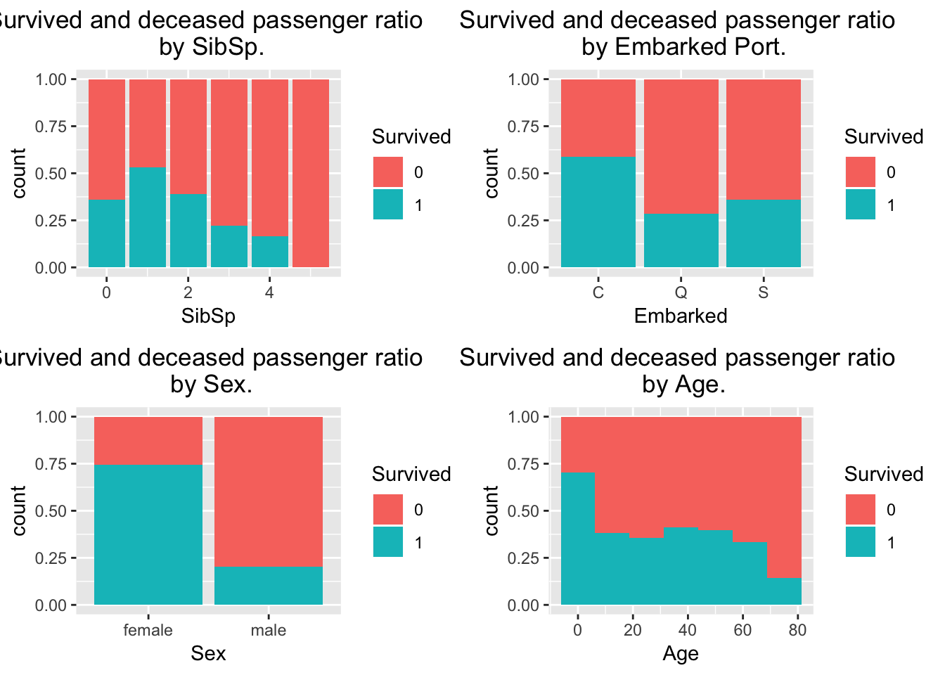
length(train[train$Fare < 200,1])/length(train[,1])

## [1] 0.9747899

Lets plot the rest of the pertinent parameters: SibSp, port of embarkment, sex, and age: First, we load gridExtra and then use it to arrange the plots in an aesthetically pleasing 2X2 form.

library(gridExtra)
p1 <- ggplot(train[train$Fare < 200,], aes(x = SibSp, fill = Survived)) + geom_bar(position = "fill", stat = "count") + ggtitle("Survived and deceased passenger ratio \n by SibSp.") + theme(plot.title = element_text(hjust = 0.5))
p2 <- ggplot(train[train$Fare < 200 & train$Embarked != "",], aes(x = Embarked, fill = Survived)) + geom_bar(position = "fill", stat = "count") + ggtitle("Survived and deceased passenger ratio \n by Embarked Port.") + theme(plot.title = element_text(hjust = 0.5))
p3 <- ggplot(train[train$Fare < 200,], aes(x = Sex, fill = Survived)) + geom_bar(position = "fill", stat = "count") + ggtitle("Survived and deceased passenger ratio \n by Sex.") + theme(plot.title = element_text(hjust = 0.5))
p4 <-ggplot(train[train$Fare < 200,], aes(x = Age, fill = Survived)) + geom_histogram(position = "fill", binwidth = 12.5) + ggtitle("Survived and deceased passenger ratio \n by Age.") + theme(plot.title = element_text(hjust = 0.5))
grid.arrange(p1,p2,p3,p4, nrow = 2)

Before we proceed to construct our model we need to impute the values. There are various methods and tools we could use to impute the missing values, in this kernel we’ll utilize the mice package. First, lets take a look at how some of our variables might indicate the passenger’s age. At first glance, we might be curious about the average (and variation) of the ages of passengers for each SibSp value ( number of siblings and spouses aboard) and parch (the number of parents/childrenaboard).

library(plotly, warn.conflicts = FALSE)
p1<- ggplot(train, aes(x = factor(SibSp), y = Age)) + geom_boxplot() 
p2<- ggplot(train, aes(x = factor(Parch), y = Age)) + geom_boxplot() 
p3<- ggplot(train, aes(x = factor(Pclass), y = Age)) + geom_boxplot()
p1h<- ggplot(train, aes(x = SibSp)) + geom_histogram(binwidth = 1)
p2h<- ggplot(train, aes(x = Parch)) + geom_histogram(binwidth = 1) 
p3h<- ggplot(train, aes(x = Pclass)) + geom_histogram(binwidth = 1)
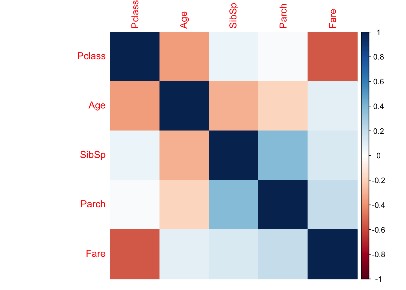
subplot(p1,p2,p3,p1h,p2h,p3h, nrows = 2,titleX = TRUE,margin = c(0,0,.075,.075))

Let’s go ahead and isolate the variables we think would best predict the age, and visualize a correlation matrix.

library(corrplot)

## corrplot 0.84 loaded

temp<- train[,-c(1,3,8)]
corrplot(cor(temp), method = "color")

From the correlation plot, we’re able to deduce that there is infact a weak correlation between Age and the variables: Pclass, SibSp, and Parch. With Pclass being the ‘strongest’ of all (albiet relatively weak). From the visualizations previous to the correlation plot, we do see some shifting in the average age between varying values of sibsp, Parch, and Pclass. I would be a bit skeptical about taking this variation seriously though, since the sample sizes for SibSp, and Parch do get smaller as those values increase.

Imputation

There are several ways we can proceede, and we will choose 3. 1. We will impute the missing age values in our dataset with the average age accross all passengers. 2. We will impute the missing age values with the average for each value of SibSp 3. We’ll utilize the mice package to find an imputation method with the least amount of RMSE. Well, how exactly can we determine the RMSE for the current missing values? We really can’t, so the next best way to approach this is to artificially impute our complete dataset with NA values, and compare it to the true complete dataset.

library(DMwR)

## Loading required package: lattice

## Loading required package: grid

set.seed(123)
impute.index <- sample(1:nrow(train), 124)
train.impute <- train
train.impute$Age[impute.index] <- NA

Now to impute the mean age into missing values.

train.meanage <- train.impute
train.meanage[is.na(train.meanage$Age),4] <- mean(na.omit(train.meanage$Age))
regr.eval(train.meanage$Age[impute.index], train$Age[impute.index])

##         mae         mse        rmse        mape 
##  11.4765016 204.5019876  14.3004191   0.3860304

Great, that gives us 1.

train.meansibsp <- train.impute
train.meansibsp[(train.meansibsp$SibSp == 0) & is.na(train.meansibsp$Age),4] <- mean(train.meansibsp[(train.meansibsp$SibSp == 0) & !is.na(train.meansibsp$Age),4])
train.meansibsp[(train.meansibsp$SibSp == 1) & is.na(train.meansibsp$Age),4] <- mean(train.meansibsp[(train.meansibsp$SibSp == 1) & !is.na(train.meansibsp$Age),4])
train.meansibsp[(train.meansibsp$SibSp == 2) & is.na(train.meansibsp$Age),4] <- mean(train.meansibsp[(train.meansibsp$SibSp == 2) & !is.na(train.meansibsp$Age),4])
train.meansibsp[(train.meansibsp$SibSp == 3) & is.na(train.meansibsp$Age),4] <- mean(train.meansibsp[(train.meansibsp$SibSp == 3) & !is.na(train.meansibsp$Age),4])
train.meansibsp[(train.meansibsp$SibSp == 4) & is.na(train.meansibsp$Age),4] <- mean(train.meansibsp[(train.meansibsp$SibSp == 4) & !is.na(train.meansibsp$Age),4])
train.meansibsp[(train.meansibsp$SibSp == 5) & is.na(train.meansibsp$Age),4] <- mean(train.meansibsp[(train.meansibsp$SibSp == 5) & !is.na(train.meansibsp$Age),4])
regr.eval(train.meansibsp$Age[impute.index], train$Age[impute.index])

##         mae         mse        rmse        mape 
##  10.9014841 185.5734764  13.6225356   0.3686145

That takes care of number 2 (the average for each value of SibSp).

library(mice, warn.conflicts = FALSE)
train.mice <- train.impute
impmethods <- c("pmm", "cart", "rf", "norm.predict", "midastouch", "sample")
for (i in 1:length(impmethods)){
  print(paste0(impmethods[i], ":"))
  miceimp <- mice(data = train.mice[, -c(3,8)], m = 3, method = impmethods[i], printFlag = F)
  micepred<- complete(miceimp)
  print(regr.eval(micepred$Age[impute.index],train$Age[impute.index]))
}

## [1] "pmm:"
##         mae         mse        rmse        mape 
##  16.1068548 372.2706653  19.2943169   0.9880562 
## [1] "cart:"
##         mae         mse        rmse        mape 
##  12.0967742 257.2409274  16.0387321   0.7610057 
## [1] "rf:"
##         mae         mse        rmse        mape 
##  12.8816935 252.8058782  15.8998704   0.9130673 
## [1] "norm.predict:"
##         mae         mse        rmse        mape 
##   9.4813373 139.9517343  11.8301198   0.3331902 
## [1] "midastouch:"
##         mae         mse        rmse        mape 
##  11.9018548 251.8903137  15.8710527   0.6532819 
## [1] "sample:"
##        mae        mse       rmse       mape 
##  16.159919 397.483862  19.936997   2.204384

The R package ‘mice’ stands for multivariate imputation by chained equations. It’s a pretty robust package that allows you to utilize various ML algorithms to impute missing values. For mice we have excluded Sex and Embarked Port, since the package ends up excluding those (either way, we previously saw that those variables correlate very little with age). The smallest root mean square error, and mean absolute percentage error we have found was with the “norm.predict” method of mice. We’ll go ahead and use that method to impute our training dataset.

train.imputed <- titanic_train[, -c(1,4,9,11)]
miceimp <- mice(data = train.imputed, m = 3, method = "norm.predict", printFlag = F)

## Warning: Number of logged events: 2

train_complete <- complete(miceimp)

Great, now that we have a complete training set, we can choose a machine learning model to train. We can go ahead and omit the passengers with missing embarked ports, which are only two. This won’t have an effect on the predictions of our test set, since there are no passengers with missing ports of embarkment in our test set.

titanic_train$Age <- train_complete$Age
titanic_train$Age <- round(train_complete$Age)
titanic_train <- titanic_train[titanic_train$Embarked != "",]

let’s impute the missing age values for our test set.

test <- read.csv(file = "../../test.csv", header = T, stringsAsFactors = F)
head(test)

##   PassengerId Pclass                                         Name    Sex
## 1         892      3                             Kelly, Mr. James   male
## 2         893      3             Wilkes, Mrs. James (Ellen Needs) female
## 3         894      2                    Myles, Mr. Thomas Francis   male
## 4         895      3                             Wirz, Mr. Albert   male
## 5         896      3 Hirvonen, Mrs. Alexander (Helga E Lindqvist) female
## 6         897      3                   Svensson, Mr. Johan Cervin   male
##    Age SibSp Parch  Ticket    Fare Cabin Embarked
## 1 34.5     0     0  330911  7.8292              Q
## 2 47.0     1     0  363272  7.0000              S
## 3 62.0     0     0  240276  9.6875              Q
## 4 27.0     0     0  315154  8.6625              S
## 5 22.0     1     1 3101298 12.2875              S
## 6 14.0     0     0    7538  9.2250              S

There is a missing fare value for one of the passengers. Instead of setting up an imputation model for one entry, let’s just assign his fare to be the mean of all third class fares. We’ll impute the missing age values as well.

test$Fare[is.na(test$Fare)]  <- mean(test$Fare[test$Pclass == 3 & !is.na(test$Fare)])
mice_test <- mice(data = test[,-c(1,3,8,10)], m = 3, method = "norm.predict", printFlag = F)

## Warning: Number of logged events: 2

test_imp <- complete(mice_test)
test$Age <- round(test_imp$Age)
 test$Pclass <- as.factor(test$Pclass)
 test$Sex <- as.factor(test$Sex)
 test$SibSp <- as.factor(test$SibSp)
 test$Embarked <- as.factor(test$Embarked)
 titanic_train$Survived <- as.factor(titanic_train$Survived)
 titanic_train$Pclass <- as.factor(titanic_train$Pclass)
 titanic_train$Sex <- as.factor(titanic_train$Sex)
 titanic_train$SibSp <- as.factor(titanic_train$SibSp)
 titanic_train$Embarked <- as.factor(titanic_train$Embarked)

We’ll be utilizing a random forest algorithm that is based on conditional inference trees. It’s called ‘cforest’ and is a part of the ‘party’ package in r. The parameters we will try to train are ntree, and mtry. We’ll set a fifth of our training set aside, and ‘scan’ the paramter space for the least amount of errors.

library(party,quietly = T)

## 
## Attaching package: 'zoo'

## The following objects are masked from 'package:base':
## 
##     as.Date, as.Date.numeric

rf.ntree <- seq(1000,2000,200)
rf.mtry <- seq(2,5,1)
sampindx <- sample(1:nrow(titanic_train), 180)
rf.train <- titanic_train[-sampindx,]
rf.test <- titanic_train[sampindx,]
param.mtry <- c()
param.ntree <- c()
param.err <- c()
for(i in 1:length(rf.mtry)){
  for(j in 1:length(rf.ntree)){
    rf.mod <- cforest(Survived ~ Fare + SibSp + Parch + Pclass + Embarked  + Sex + Age, data = rf.train[,-c(1,4,9,11)], controls = cforest_unbiased(mtry = rf.mtry[i], ntree = rf.ntree[j]))
    param.mtry <- c(param.mtry, i)
    param.ntree <- c(param.ntree, rf.ntree[j])
    err <- sum(abs(as.numeric(rf.test$Survived) - as.numeric(predict(rf.mod, newdata = rf.test[,-c(1,4,9,11)], OOB = TRUE, type = "response"))))/nrow(rf.test)
    param.err <- c(param.err,err)
  }
}
rf.results <- data.frame(cbind(param.ntree,param.mtry,param.err))

let’s go ahead and plot the error results in our parameter space!

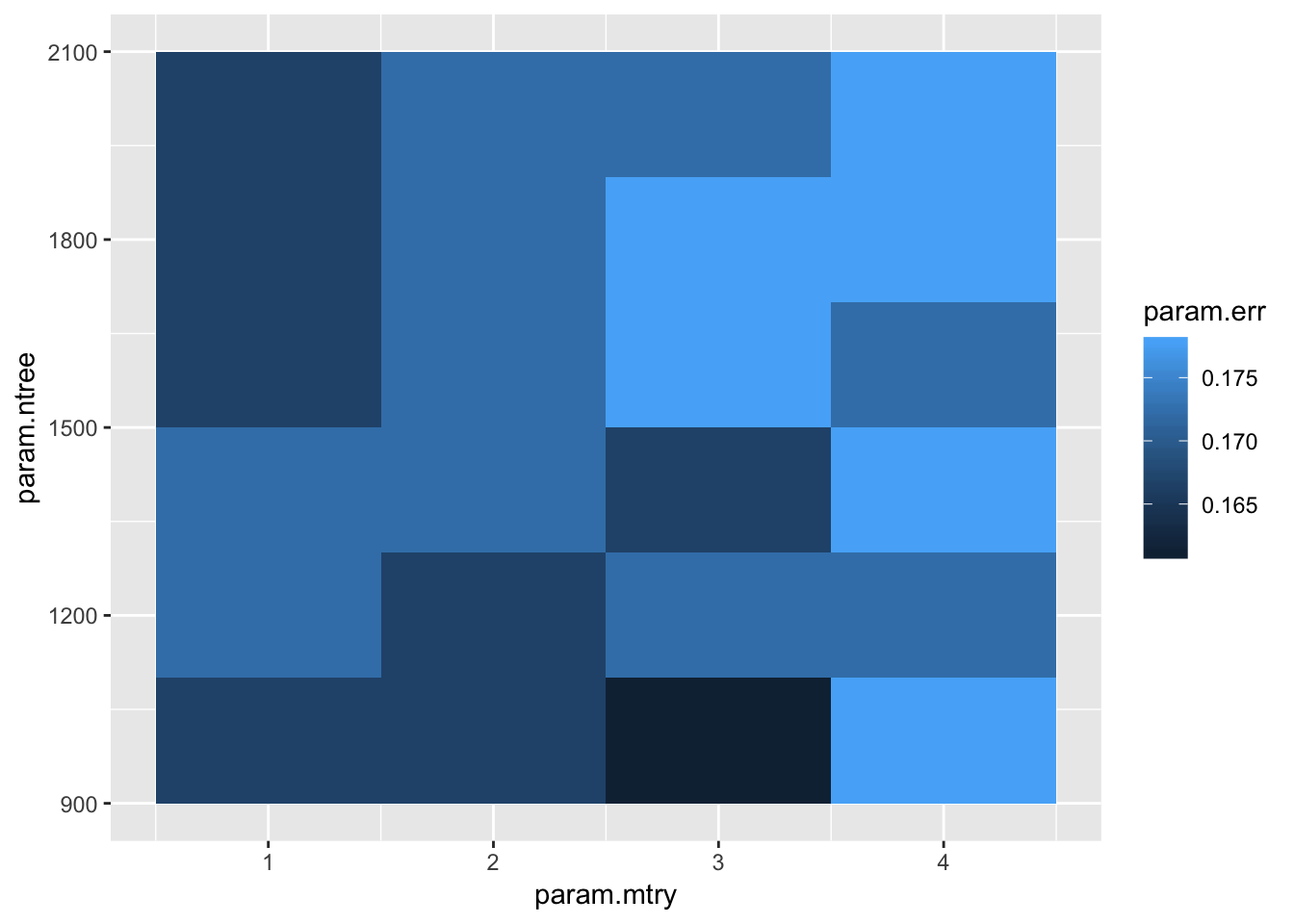
ggplot(data = rf.results, aes(x = param.mtry, y = param.ntree, z = param.err)) + geom_tile(aes(fill = param.err))

Lets go with mtry = 3, and ntree = 2000. That seems to give us the least amount of error.

    rf.mod <- cforest(Survived ~ Fare + SibSp + Parch + Pclass + Embarked  + Sex + Age, data = titanic_train[,-c(1,4,9,11)], controls = cforest_unbiased(mtry = 3, ntree = 2000))
test.results <- predict(rf.mod, newdata = test[,-c(1,3,8,10)], OOB = TRUE, type = "response")
test$Survived <- test.results

Afterwards, we just write our results out as a csv, and check the results on kaggle!

write.csv(test[1,12], file = "../../../Results.csv", row.names = FALSE)

Hey, not bad! 5333 out of 10500 with a 78% accuracy. It’s not the top 10%, but it’s certainly nothing to scoff at. Of course, there are other ways we could “extract” features from our data. I’m not quite sure what my next blog post will be about. I’ve been reading up on some of the sensors available for arduino, and I’m certain I’d be able to extract some interesting raw data out of those sensors. As of yet I haven’t made any concrete commitment to a particular project, but if you have any ideas I’m all ears!