Predicting Missed Transcriber Deadlines With SciKit-Learn ML Classifiers.
Intro
Hey there! It’s been a while since muy previous update. In that update, I mentioned the fact that
I relocated to Seattle. I accepted a position as a Data Analyst/ BI Engineer. Fortunately, this position allowed
me to quickly adopt Python, and become more fluent and agile with Pandas in the context of Data Analytics.
I still prefer R, but it’s hard to ignore all of the cool and exciting libraries and frameworks available for Python.
This has lead me to become determined in increasing my fluency in Python.
Recently, I took a course on Datacamp that detailed utilizing the sci-kit learn package for machine learning classification
and regression. I’m not new to machine learning. In fact, you can find a few articles in this blog on that topic.
In R my tool of choice was the Caret library. However, after completing the course I was surprised to see that a
large portion of the pre-processing, model selection and tuning is just as easy in sci-kit learn as it is in Caret.
I thought I’d use my new skills in sci-kit learn, by outlining how to train a machine learning
classification model on some interesting data.
To me, the most interesting data is data that is impactful and can drive some type of change.
Recently, I came accross some data on Kaggle for Rev.com’s transcribing service.
This dataset contained several metrics measuring job level attributes of customers and agents.
In this article, we’ll identify pertinent variables and measurements that will allow us to predict whether
(if an agent accepts or chooses the job) an agent will meet or exceed the deadline set
by the customer. This can allow rev.com to emphasize particular jobs to agents they think will be able to meet the job’s deadline.
We’ll do this by
Introducing the data set, checking for nulls and cleanliness.
Performing some EDA.
Carrying out a bit of Feature Engineering.
Training and Testing two models utilizing GLM & Random Forest.
Data and Background
A table providing meta-data about the dataset, as well as the table is printed below.
This dataset is essentailly a log of 20 thousand jobs fulfilled by rev.com agents (reffered to as revvers).
Each job record (row) contains the JobID, data about when the Job was started, completed, it’s expected duration, and when the job was due.
There is also some agent-level data like the agent’s rev.com level when the job was accepted, and the particular agent’s ID.
The only customer data is the ID of the customer that submitted the job. Finally we have two metrics of interest, the elapsed amount of time in
seconds after the deadline (negative for jobs fulfilled within the deadline) and whether it was fulfilled within the specified deadline.
rev_df.info()## <class 'pandas.core.frame.DataFrame'>
## RangeIndex: 20022 entries, 0 to 20021
## Data columns (total 25 columns):
## # Column Non-Null Count Dtype
## --- ------ -------------- -----
## 0 JobId 20022 non-null int64
## 1 JobStartedOnTS 20022 non-null datetime64[ns]
## 2 JobStartedOnDay 20022 non-null int64
## 3 JobStartedOnWeekday 20022 non-null int64
## 4 JobStartedOnHour 20022 non-null int64
## 5 JobStartedOnMinute 20022 non-null int64
## 6 JobCompletedOnTS 20022 non-null datetime64[ns]
## 7 JobCompletedOnDay 20022 non-null int64
## 8 JobCompletedOnWeekday 20022 non-null int64
## 9 JobCompletedOnHour 20022 non-null int64
## 10 JobCompletedOnMinute 20022 non-null int64
## 11 JobDueOnTS 20022 non-null datetime64[ns]
## 12 JobDueOnWeekday 20022 non-null int64
## 13 JobDueOnDay 20022 non-null int64
## 14 JobDueOnHour 20022 non-null int64
## 15 JobDueOnMinute 20022 non-null int64
## 16 AgentLevelWhenJobClaimed 20022 non-null int64
## 17 ProjectLengthSeconds 20022 non-null int64
## 18 ProjectLengthSegment 20022 non-null int64
## 19 CustomerId 20022 non-null int64
## 20 AgentId 20022 non-null int64
## 21 ExpectedJobDurationSeconds 20022 non-null int64
## 22 ActualJobDurationSeconds 20022 non-null int64
## 23 ElapsedSecondsAfterDueOn 20022 non-null int64
## 24 DeadlineRespected 20022 non-null bool
## dtypes: bool(1), datetime64[ns](3), int64(21)
## memory usage: 3.7 MBFortunately, our dataset does not contain any nulls and appears to be pretty clean.
We can get a better idea of the dataset by printing out the dataset header.
##     JobId      JobStartedOnTS JobStartedOnDay JobStartedOnWeekday
## 1 1801338 2016-01-07 13:48:00               7                   5
## 2 1793811 2016-01-06 05:58:00               6                   4
## 3 1813562 2016-01-11 11:50:00              11                   2
## 4 1807190 2016-01-08 17:48:00               9                   7
## 5 1865366 2016-01-23 14:09:00              23                   7
## 6 1828095 2016-01-14 09:41:00              14                   5
##   JobStartedOnHour JobStartedOnMinute    JobCompletedOnTS JobCompletedOnDay
## 1               21                 48 2016-01-09 12:34:00                 9
## 2               13                 58 2016-01-06 06:43:00                 6
## 3               19                 50 2016-01-12 06:04:00                12
## 4                1                 48 2016-01-14 08:10:00                14
## 5               22                  9 2016-01-23 14:09:00                23
## 6               17                 41 2016-01-14 12:53:00                14
##   JobCompletedOnWeekday JobCompletedOnHour JobCompletedOnMinute
## 1                     7                 20                   34
## 2                     4                 14                   43
## 3                     3                 14                    4
## 4                     5                 16                   10
## 5                     7                 22                    9
## 6                     5                 20                   53
##            JobDueOnTS JobDueOnWeekday JobDueOnDay JobDueOnHour JobDueOnMinute
## 1 2016-01-09 15:58:00               2           9           23             58
## 2 2016-01-06 07:28:00               4           6           15             28
## 3 2016-01-13 19:20:00               4          14            3             20
## 4 2016-01-14 04:58:00               4          14           12             58
## 5 2016-01-23 18:39:00               4          24            2             39
## 6 2016-01-14 20:51:00               4          15            4             51
##   AgentLevelWhenJobClaimed ProjectLengthSeconds ProjectLengthSegment CustomerId
## 1                        1                 5340                    5     140440
## 2                        2                  180                    1     159507
## 3                        2                 6300                    5     185608
## 4                        1                14520                    6      75334
## 5                        2                  720                    3     191231
## 6                        2                 1920                    4     206837
##   AgentId ExpectedJobDurationSeconds ActualJobDurationSeconds
## 1  194641                     180600                    81960
## 2  170003                       5400                     2700
## 3  105819                     199800                    65640
## 4  198256                     472200                    51720
## 5  190339                      16200                        0
## 6  101595                      40200                    11520
##   ElapsedSecondsAfterDueOn DeadlineRespected
## 1                   -12240              TRUE
## 2                    -2700              TRUE
## 3                  -134160              TRUE
## 4                    11520             FALSE
## 5                   -16200              TRUE
## 6                   -28680              TRUE
Before we jump into any kind of ML training we should look at the response variable proportions. This will give us some general overview as to how balanced our response variable is.
deadline_counts_df = rev_df.groupby(["DeadlineRespected"], as_index = False).\
            agg(count = pd.NamedAgg("DeadlineRespected", "count"))

deadline_counts_fig = ggplot(deadline_counts_df, aes(x = "DeadlineRespected", y = "count", fill = "DeadlineRespected")) +\
      geom_col() +\
        theme_minimal()

deadline_counts_fig.draw()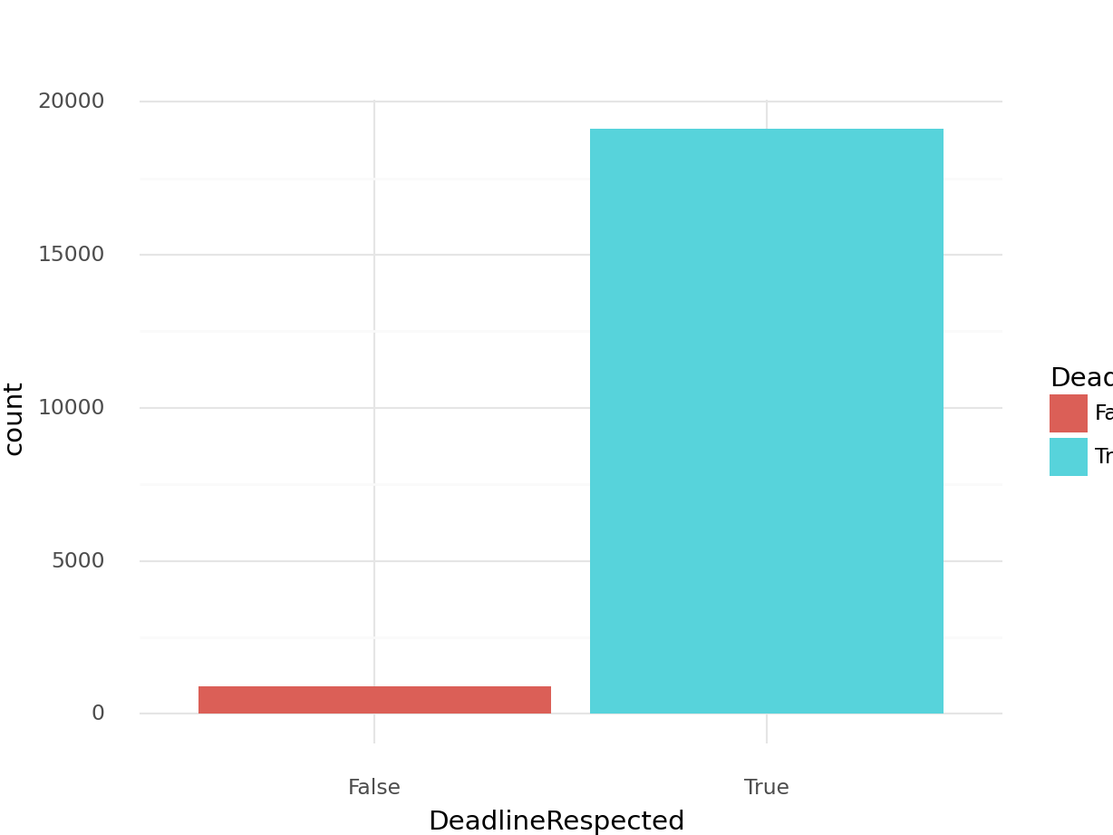
deadline_counts_df## DeadlineRespected count
## 0 False 914
## 1 True 19108Yikes, our dataset is extremely unbalanced. We’ll have to make sure we address this later by stratifying our CV splits,
as well as our training and test set to account for this.
Next, we can take a look at the AgentLevel of revvers that failed to meet deadlines.
agent_level_counts_df = rev_df.\
            groupby(["AgentLevelWhenJobClaimed", "DeadlineRespected"], as_index = False).\
            agg(count = pd.NamedAgg("AgentLevelWhenJobClaimed", "count"))
#agent_level_counts_df = agent_level_counts_df.assign(AgentLevelWhenJobClaimed = lambda x: np.where(x["AgentLevelWhenJobClaimed"] == 0, "Zero", np.where(x["AgentLevelWhenJobClaimed"] == 1, "One", "Two")))

agent_level_deadline_fig = ggplot(agent_level_counts_df,
           aes(x = "DeadlineRespected",
                y = "count",
                fill = "AgentLevelWhenJobClaimed")) +\
           geom_col(position = "fill")

agent_level_deadline_fig.draw()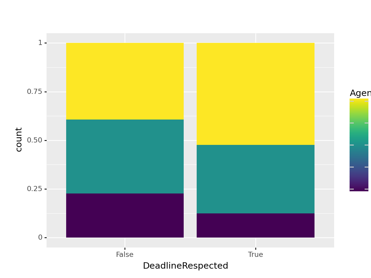
It seems like agents in the bottom two revver levels account for more of the revvers that failed to meet deadlines, but it doesn’t seem like it’s significantly more. We might also be interested in the the distributions of the expected job durations for jobs that resulted in met and exceeded deadlines. We’ll remove all outliers in this visualization, as some extreme outliers skew the figure, effectively compressing the boxplots.
deadline_exp_job_duration_fig = ggplot(rev_df, aes(y = "ExpectedJobDurationSeconds", x= "DeadlineRespected")) +\
geom_boxplot(outlier_shape = "") +\
ylim(0,20e4)
deadline_exp_job_duration_fig.draw()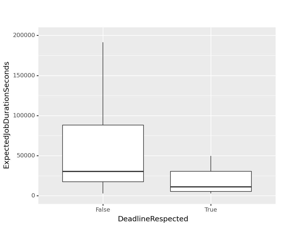 This is interesting. It seems like the distribution of jobs that resulted in missed deadlines skew larger than the jobs where deadlines were met. This could be due to revvers underestimating the amount of time it would take to complete a deadline. All assumptions aside, this is an interesting metric we should include in our ML model.
Feature Engineering
Unfortunately, outside of our response variable, and a couple of explanatory variables not much of our dataset can be directly used in an ML model as-is. This is where we have to get a little creative, and engineer some explanatory variables utilizing the data we do have. This is a classic real-world example. When you obtain a raw data-set it is rarely (if ever) plug-and-play ready for training a ML model.
First, let’s take a step back and re-examine variables we have, so we can determine what kind of features we can create utilizing them. Since our dataset is essentially a log of jobs fulfilled by revvers, we can extract not only the number of jobs a revver has completed, but the number of jobs they’ve claimed which exceeded deadlines. Furthermore, we have the the revver’s record of prior time difference between deadline and job submissions, as well as their prior history of estimated job durations for jobs they have claimed in the past. We can use all of these metrics to calculate some measure of deadline delinquency and job length ‘over-extention’ by measuring the difference between the current accepted job, and previous job durations.
Let’s get started, first we’ll feature engineer the count of previous jobs fulfilled by the revver, and the count of previous jobs where they failed to meet the deadline:
### Count number of previous jobs completed by Rev Agent.
rev_df["NPrevJob"] = rev_df.\
            sort_values(["AgentId", "JobStartedOnTS"]).\
            groupby(["AgentId"], as_index = False).cumcount()


### Count number of previous jobs where Agent missed deadline.
rev_df = rev_df.\
            assign(NOverDeadline =\
                   lambda x: np.where(x["DeadlineRespected"] == False, 1, 0))

rev_df["NOverDeadline"] = rev_df.\
            sort_values(["AgentId", "JobStartedOnTS"]).\
            groupby(["AgentId"], as_index = False)["NOverDeadline"].\
            cumsum()

rev_df = rev_df.\
            assign(NOverDeadline = lambda x:
                   np.where(x["DeadlineRespected"] == False,
                            x["NOverDeadline"] - 1,
                            x["NOverDeadline"]))

rev_df = rev_df.sort_values(["AgentId", "JobStartedOnTS"]).reset_index(drop = True)
Let’s print a trimmed header of the result, if we focus on a particular revver we can see if our logic is correct.
##        JobStartedOnTS   JobId AgentId CustomerId DeadlineRespected NPrevJob
## 1 2016-01-03 14:13:00 1782287   27006     196251              TRUE        0
## 2 2016-01-06 13:46:00 1795818   27006      75334             FALSE        1
## 3 2016-01-17 19:18:00 1839780   27006     170329             FALSE        2
## 4 2016-01-19 16:00:00 1846606   27006     170329              TRUE        3
## 5 2016-01-22 18:26:00 1862726   27006     170329             FALSE        4
##   NOverDeadline
## 1             0
## 2             0
## 3             1
## 4             2
## 5             2
Awesome! For the revver with AgentId 27006, we see that the variables NPrevJob, and NOverDeadline display the correct results.
Let’s take a look at the two features we just created, and how they interact with jobs that end in missed deadlines.
We can plot a basic barchart using “NOverDeadline”, and see how many revvers with
missed deadlines have a record of previously missing deadlines.
deadlines_missed_counts_df = rev_df[rev_df["DeadlineRespected"] == False].\
        assign(NOverDeadline = lambda x: np.where(x["NOverDeadline"] < 1, "0",
                                                 np.where(x["NOverDeadline"] < 10, "1-10", "GT10"))).\
        groupby("NOverDeadline", as_index = False).\
        agg(CountJobOverDeadline = pd.NamedAgg("NOverDeadline", "count"))


deadlines_missed_count_fig = ggplot(deadlines_missed_counts_df,aes(x = "NOverDeadline", y = "CountJobOverDeadline")) +\
                geom_col() +\
                theme_538() +\
                xlab("Previous Deadlines Missed") +\
                ylab("Jobs With Missed Deadlines (Count)") +\
                ggtitle("Count of Jobs with Missed Deadlines \n by Previous Deadlines Missed by Agent")

deadlines_missed_count_fig.draw()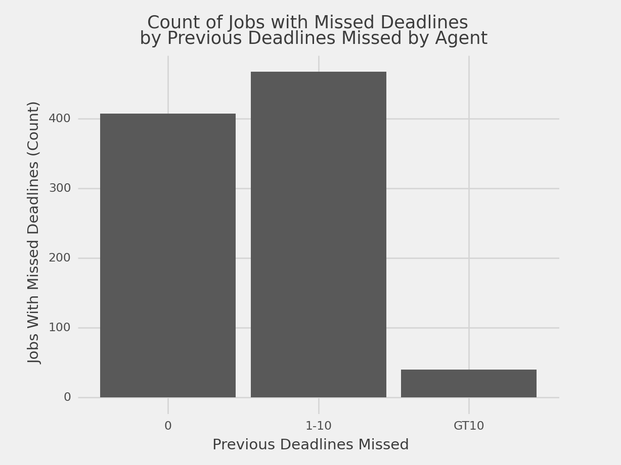
So marginally more jobs that resulted in missed deadlines were submitted
by agents with previous missed deadlines.
Let’s see what the number of previous jobs submitted by revvers tells us about missed deadlines.
We’ll do this by separating jobs by DeadlineRespected, and plot the number of previous jobs fulfilled by the revver
via boxplots.
nprevjob_missed_deadlines_fig = ggplot(rev_df, aes(x = "DeadlineRespected", y = "NPrevJob"))  +\
            geom_boxplot(outlier_shape = "") +\
            ylim(0,60) + \
            ggtitle("Previous Jobs Completed by Deadline Respected")

nprevjob_missed_deadlines_fig.draw()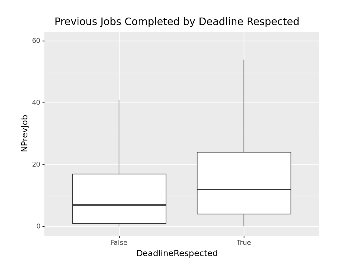
It seems like a large majority of jobs that resulted in missed deadlines were submitted by revvers with
a smaller number of previous jobs fulfilled. This coule be a direct result of inexperience, or poor time
management.
Let’s get to the rest of the features we’re going to create. We just found a way to measure not only
how many jobs a revver has previously accepted, but the number of jobs where they exceeded the deadline.
Fortunately, we also have a record of the revver’s measured duration in completing their previous job, and the
expected job duration when they accepted the job.
Using these two variables, we can create a metric that compares the current expected job duration, and an aggregate measure of the revvers previous job durations. To do this, we’ll use an informal version of a z-score. We’ll calculate an expanding average of previous job durations, as well as the expanding standard deviation. With these two metrics, we can calculate how many standard deviations the current expected job duration is from the mean.
We’ll also follow the same methodology for measuring the z-score for a revver’s previous expected job duration, and the current expected job duration, and count the number of jobs previously submitted by customers that have resulted in missed deadlines.
### Calculate running standard deviation and average, for expected durations of previous jobs.
rev_df["StdExp"] =  rev_df.sort_values(["AgentId", "JobStartedOnTS"]).groupby(["AgentId"], as_index = False)["ExpectedJobDurationSeconds"].expanding().std().reset_index(drop = True)

rev_df["AvgExp"] = rev_df.sort_values(["AgentId", "JobStartedOnTS"]).groupby(["AgentId"], as_index = False)["ExpectedJobDurationSeconds"].expanding().mean().reset_index(drop = True)

### Calculate the z-score for the job of interest using running standard deviation and mean of previously accepted jobs.
rev_df = rev_df.assign(StdExp = lambda x: np.where(x["StdExp"].isna(), 0, x["StdExp"])).\
       assign(ZScore = lambda x: (x["ExpectedJobDurationSeconds"] - x["AvgExp"])/x["StdExp"]).\
       assign(ZScore = lambda x: np.where((x["ZScore"].isna()) | (x["StdExp"] == 0), 0, x["ZScore"]),
              DeadlineRespected = lambda x: np.where(x["DeadlineRespected"] == True, 1, 0))

### Count number of previously submitted jobs by customer that has ended in non-fulfillment within deadline.
rev_df = rev_df.assign(CustomerNOverDeadline = lambda x: np.where(x["DeadlineRespected"] == 0, 1, 0))
rev_df["CustomerNOverDeadline"] = rev_df.sort_values(["JobStartedOnTS", "CustomerId"]).groupby(["CustomerId"], as_index = False)["CustomerNOverDeadline"].cumsum()
### Calculate the actual job duration.

rev_df["ActStdExp"] =  rev_df.sort_values(["AgentId", "JobStartedOnTS"]).\
                    groupby(["AgentId"], as_index = False)["ActualJobDurationSeconds"].\
                    expanding().\
                    std().\
                    groupby(level = 0).\
                    shift().\
                    reset_index(drop = True).\
                    fillna(0)

rev_df["ActAvgExp"] = rev_df.sort_values(["AgentId", "JobStartedOnTS"]).\
                    groupby(["AgentId"], as_index = False)["ActualJobDurationSeconds"].\
                    expanding().\
                    mean().\
                    groupby(level = 0).\
                    shift().\
                    reset_index(drop = True).\
                    fillna(0)


rev_df["AvgSubBeforeDeadline"] = rev_df.sort_values(["AgentId", "JobStartedOnTS"]).\
                    groupby(["AgentId"], as_index = False)["ElapsedSecondsAfterDueOn"].\
                    expanding().\
                    mean().\
                    groupby(level = 0).\
                    shift().\
                    reset_index(drop = True).\
                    fillna(0)

rev_df = rev_df.assign(ActZScore = lambda x:\
                                       np.where(x["ActStdExp"] == 0,
                                                0,
                                                (x["ExpectedJobDurationSeconds"] - x["ActStdExp"])/(x["ActStdExp"])))
First, we sort by AgentId, and JobStartedOnTS, and then we group by AgentId and take the expanding standard deviation of the previous expected job durations, (not including the current one). We use the same process to obtain the mean expected duration of previous jobs. Both of these metrics, and the current expected job duration is all we need to obtain a ZScore. We follow an identical process to obtain ActZScore which is the ZScore of the current expected job duration against the actual durations of previous jobs.
Let’s take a look and see how our response variable varies with these two metrics. We’ll do this by generating two separate boxplots for each individual class of DeadlineRespected, filtering outliers out of the visualization to avoid skewing.
z_score_prev_exp_fig = ggplot(rev_df.assign(DeadlineRespected = lambda x:\
                     np.where(x["DeadlineRespected"].astype(str) == "1", "Yes", "No")),\
                   aes(x = "DeadlineRespected", y = "ZScore")) +\
                    geom_boxplot(outlier_shape = "") +\
                    xlab("Deadline Respected") +\
                    ylab("Expected Deadline Length Z Score") + \
                    ggtitle("Z-Score of Current Expected Deadline\n Against Previously Expected Deadlines ") +\
                    ylim(-2.5,3)

z_score_prev_exp_fig.draw()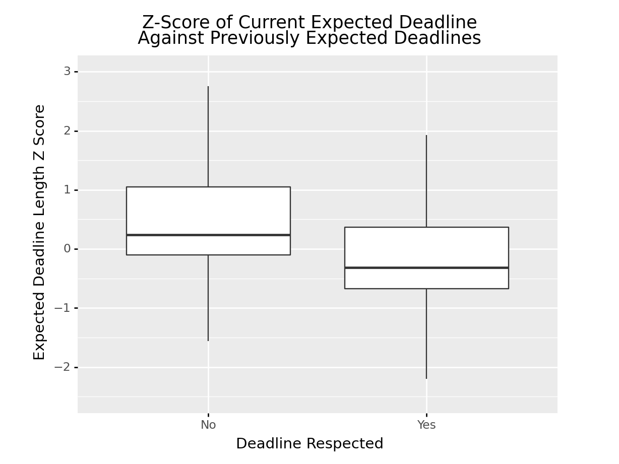
z_score_prev_exp_fig = ggplot(rev_df.assign(DeadlineRespected = lambda x:\
                     np.where(x["DeadlineRespected"].astype(str) == "1", "Yes", "No")),\
                   aes(x = "DeadlineRespected", y = "ActZScore")) +\
                    geom_boxplot(outlier_shape = "") +\
                    xlab("Deadline Respected") +\
                    ylab("Expected Deadline Length Z Score") + \
                    ggtitle("Z-Score of Current Expected Deadline\n Against Previous Actual Job Durations") +\
                    ylim(-5,12)

z_score_prev_exp_fig.draw()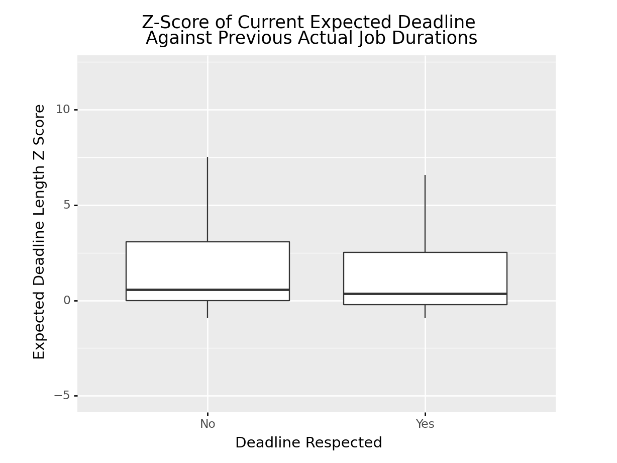
It’s apparent that ZScore is shifted higher for jobs that failed to meet deadlines. This is the ZScore of the current job’s expected duration against the previous expected job durations claimed by the revver. The shift tells us that substantial number of jobs that ended in deadlines being exceeded were longer than the previous durations of the jobs claimed by the revver.
Unfortunately, there’s not much deviation with ActZScore but we’ll include it either way for good measure.
Model Training and Testing.
Now that we have created our new metrics, it’s time to train our models! In this article we’ll be using the GLM and Random Forest algorithms to create our classification models. First, we’ll go ahead and trim away any variables that aren’t pertinent to our model, afterwords we’ll double check and make sure our dataset is void of nulls.
mod_rev_df = rev_df.loc[:,["AgentLevelWhenJobClaimed",
                           "ProjectLengthSeconds",
                           "ProjectLengthSegment",
                           "ExpectedJobDurationSeconds",
                           "NPrevJob",
                           "NOverDeadline",
                           "StdExp",
                           "ZScore",
                           "CustomerNOverDeadline",
                           "DeadlineRespected",
                           "ActZScore",
                           "ActAvgExp",
                           "ActStdExp",
                          "AvgSubBeforeDeadline"]]

mod_rev_df.isna().sum()
## AgentLevelWhenJobClaimed 0
## ProjectLengthSeconds 0
## ProjectLengthSegment 0
## ExpectedJobDurationSeconds 0
## NPrevJob 0
## NOverDeadline 0
## StdExp 0
## ZScore 0
## CustomerNOverDeadline 0
## DeadlineRespected 0
## ActZScore 0
## ActAvgExp 0
## ActStdExp 0
## AvgSubBeforeDeadline 0
## dtype: int64Fantastic. Let’s print out a header of our dataset.
##   AgentLevelWhenJobClaimed ProjectLengthSeconds ProjectLengthSegment
## 1                        2                  600                    3
## 2                        1                 1020                    3
## 3                        1                  600                    3
## 4                        1                  720                    3
## 5                        1                  278                    1
## 6                        1                 1440                    3
##   ExpectedJobDurationSeconds NPrevJob NOverDeadline   StdExp     ZScore
## 1                      13800        0             0    0.000  0.0000000
## 2                      22200        0             0    0.000  0.0000000
## 3                      13800        1             0 5939.697 -0.7071068
## 4                      16200        2             0 4326.662 -0.2773501
## 5                       6600        3             0 6452.906 -1.2552483
## 6                      30600        4             0 9043.893  1.4064740
##   CustomerNOverDeadline DeadlineRespected ActZScore ActAvgExp ActStdExp
## 1                     7                 1  0.000000         0     0.000
## 2                    47                 1  0.000000         0     0.000
## 3                    52                 1  0.000000     13860     0.000
## 4                     1                 1  2.602242     10680  4497.199
## 5                     2                 1  1.069464     10540  3189.232
## 6                    10                 1  5.607099      8625  4631.382
##   AvgSubBeforeDeadline
## 1                    0
## 2                    0
## 3                -8340
## 4                -7320
## 5                -6860
## 6                -6075
Next, we’ll separate our explanatory and response variables into numpy objects named X and y respectively. The Sci-Kit Learn package only accepts data in the numpy array type. The explanatory variables must be in MxN dimensions where N is the number of explanatory variables and M is the number of rows (or observations). The response variable y is an M x 1 array. Obtaining the data in this datatype is no big deal, as we can just drop the response variable from our dataset, and use the values attribute to obtain X. For y, we can limit our scope to the response variable solely, and use the value attribute again.
X = mod_rev_df.drop(columns="DeadlineRespected").values
y = mod_rev_df.DeadlineRespected.values
X = sk_preprocessing.scale(X)
We’ll make sure to scale our response variables to avoid any issues that could occur due to outliers in our data set. Finally, we’ll split our data set into training and testing data sets, and define some parameters to train across. We’ll be using the GridSearchCV function in SKLearn that takes a parameter grid as an argument, the estimator object, and the number of cross validation folds. We’ll opt to use a 10-fold cross validation scheme.
Finally, we’ll fit our model with the fit method, supplying our training explanatory and response variables respectively.
X_train, X_test, y_train, y_test =\
          sk_model_selection.train_test_split(X, y, stratify= y,train_size=0.85, random_state= 991)

c_space = np.logspace(-5, 8, 15)
param_grid = {"C": c_space, "penalty": ['l2']}
logreg = sk_linear_model.LogisticRegression(max_iter = 1000)

logreg_cv = sk_model_selection.GridSearchCV(logreg, param_grid, cv = 10,verbose=0)

logreg_cv.fit(X_train, y_train)
## GridSearchCV(cv=10, estimator=LogisticRegression(max_iter=1000),
##              param_grid={'C': array([1.00000000e-05, 8.48342898e-05, 7.19685673e-04, 6.10540230e-03,
##        5.17947468e-02, 4.39397056e-01, 3.72759372e+00, 3.16227766e+01,
##        2.68269580e+02, 2.27584593e+03, 1.93069773e+04, 1.63789371e+05,
##        1.38949549e+06, 1.17876863e+07, 1.00000000e+08]),
##                          'penalty': ['l2']})
The output is a print-out of all parameters GridSearchCV used to train your model, it finds the best parameters across these and automatically defaults to use those parameters.
logreg_cv.best_params_## {'C': 0.0007196856730011522, 'penalty': 'l2'}All that’s left is to assess the resulting model! The standard metric for assessing how effective a dichotomous classification model is, is the ROC’s (Receiver Operator Characteristic) area under curve. First, we’ll visualize the ROC for our GLM model.
y_pred = logreg_cv.predict(X_test)
y_score = logreg_cv.predict_proba(X_test)[:,1]


fpr, tpr, thresholds = sk_metrics.roc_curve(y_test, y_score, pos_label = 1)
roc_dict = {"fpr": fpr,
            "tpr": tpr,
            "thresholds": thresholds}
roc_df = pd.DataFrame(roc_dict)

glm_roc_df = ggplot(roc_df, aes(x = "fpr", y = "tpr")) +\
        geom_line() +\
        geom_abline(aes(slope = 1, intercept = 0), color = "red")

glm_roc_df.draw()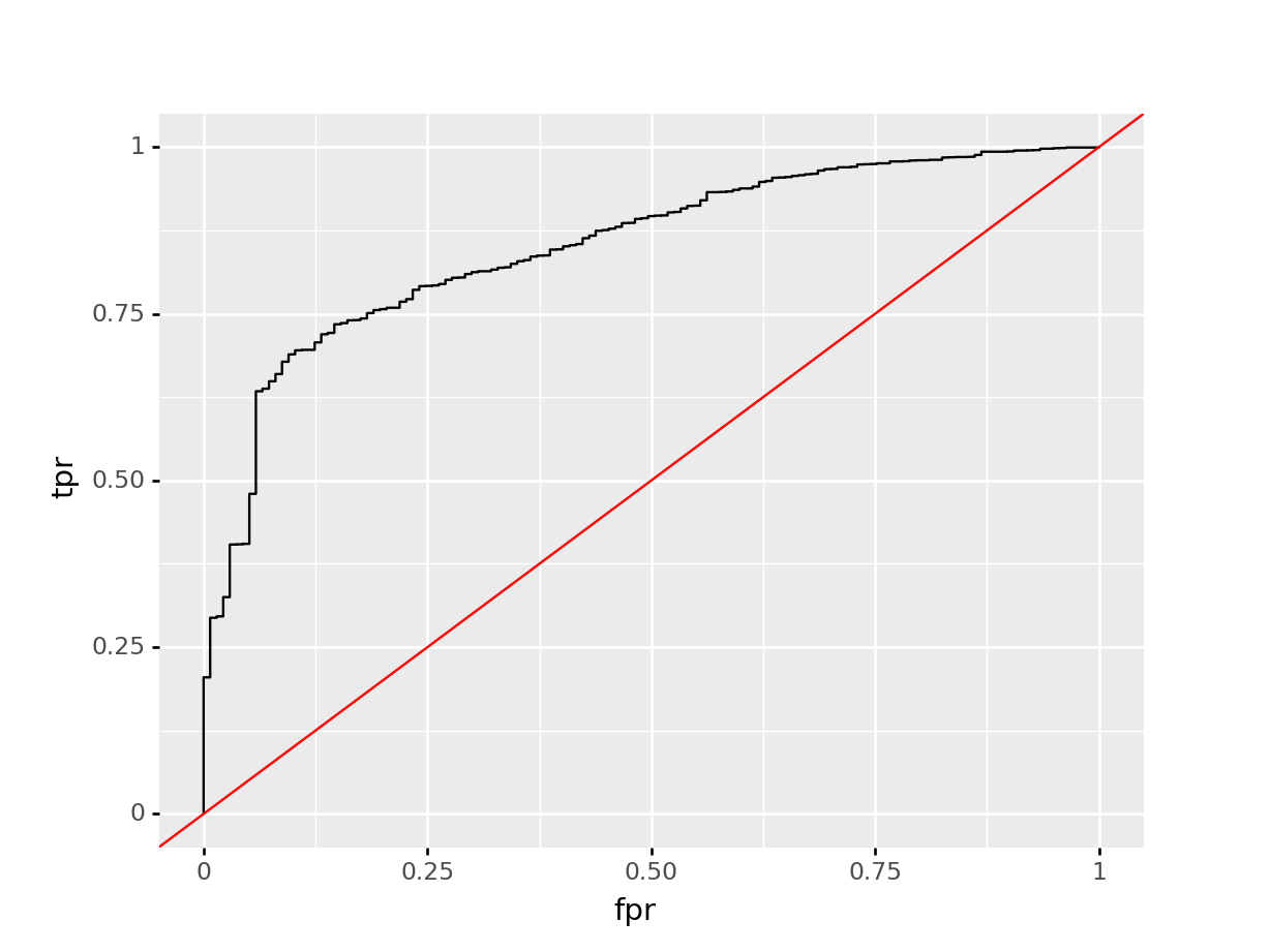
We can easily retreive the AUC by utilizing the roc_auc_score function, and supplying the test set response variable, and the predicted probabilities obtained by the model.
sk_metrics.roc_auc_score(y_test, y_score)## 0.8519001779626711Random Forest
Training our random forest model is relatively similar. The only difference here is the specified parameter grid we’ll be training across. In this instance, we’ll vary our n_estimators which indicates the amount of decision trees in our model. We’ll use the gini criterion, and select auto for max features.
n_estimators = np.arange(500,800,100)
criterion = ["gini"]
max_features = ["auto"]
param_grid_rf = {"n_estimators":n_estimators,
                "criterion":criterion,
                "max_features":max_features}

rf_class = sk_ensemble.RandomForestClassifier()
rf_cv = sk_model_selection.GridSearchCV(rf_class, param_grid_rf, cv = 10)
rf_cv.fit(X_train,y_train)
## GridSearchCV(cv=10, estimator=RandomForestClassifier(),
## param_grid={'criterion': ['gini'], 'max_features': ['auto'],
## 'n_estimators': array([500, 600, 700])})Let’s take a quick peak at our ROC plot, and print our ROC AUC.
y_prob = rf_cv.predict_proba(X_test)[:,1]
fpr, tpr, thresholds = sk_metrics.roc_curve(y_test, y_prob, pos_label = 1)
roc_dict = {"fpr": fpr,
            "tpr": tpr,
            "thresholds": thresholds}
roc_df = pd.DataFrame(roc_dict)
ggplot(roc_df, aes(x = "fpr", y = "tpr")) + geom_line() + geom_abline(aes(slope = 1, intercept = 0), color = "red")
## <ggplot: (339736284)>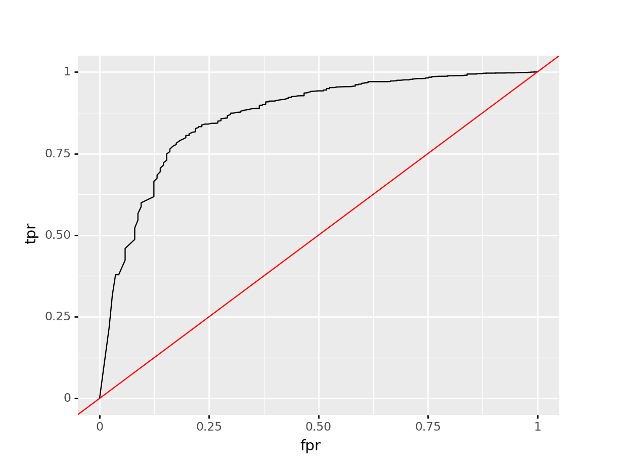
sk_metrics.roc_auc_score(y_test, y_prob)## 0.8639502111874617Not bad! A marginal improvement over our GLM model.
Conclusion & future work.
In this article, we managed to explore the underlying data set that would inform our model. We checked to make sure it was void of nulls, and examined some metrics to assess if they offered any value towards predicting our response variable. Since our data set wasn’t readily useful for modeling, we created some simple metrics based off of revver agent’s prior work. Subsequently, we utilized those metrics to create a model using Logistic Regression, and Random Forest algorithms from Sci-Kit Learn, where we found that the ROC AUC for the random forest model was marginally higher than our logistic regression model.
This model could be easily employed in a production environment to de-emphasize or restrict particular jobs to a revver when the model predicts that the revver has a high probability of failing to meet the deadline. Since this model heavily relies on a revver’s prior work, this model could be restricted to revers with a minimum amount of completed jobs.