Introduction to Programming in R: Writing and Calling Functions

Introduction

When it comes to programming, R isn’t the first language that pops into your head. It’s primary use is as a language for statistical computing, data analysis and visualization. R’s beginnings stem from another old statistical computing language created in the late 1970’s called ‘S’. According to R’s website (R Project)[https://www.r-project.org/] a large portion of code written for ‘S’ can still be run un-altered in R. The immeasurable quantity of machine learning, statistical, and data visualization packages on CRAN (Comprehensive R Archive Network), means you’ll hardly ever have to write code to implement a ML algorithm, or calculate statistical metrics.

There are incentives for learning to write functions in R though. If you’re repeatedly performing similar analysis or visualization schemes on the same set of data or data with identical structures, writing functions can help cut down on the time spent altering elements in your code. In this article I’ll go over the process of writing functions in R. I’ll cover the basic syntax, arguments (mandatory, optional, and default), as well as how to return an object (like a number, ggplot object, dataframe, or an array).

An Intro To Functions

This is the standard syntax of a function in R:

function_name <- function(arg1, arg2){
## Code Goes Here
}

Arguments

It’s worth noting that you do not have to declare the class of the arguments when creating your function, but an error will still be thrown by R if your function performs an operation that results in one. As an illustration, let’s take a look at a function that returns $A^{B}$.

expnt <- function(base, exponent){
  return(base**(exponent))
}

expnt(2,4)

## [1] 16

You don’t have to supply the arguments to the function in order, as long as you explicity name the argument when calling the function. If you explicitly name all of the arguments, the unnamed arguments will be resolved in the same order as the function statement.

expnt(3, base = 5)

## [1] 125

Another thing to keep in mind, is that while you don’t have to explicitly state what to return, it’s always considered to be a good practice. It improves the clarity of your code. If you don’t it’s not a problem, R will just return the last expression evaluated.

expnt <- function(base, exponent){
  base + exponent
  base**(exponent)
}

expnt(5,2)

## [1] 25

Functions behave differently depending on the class of arguments that are used in the call. In our previous example, we declared expnt with the purpose of exponentiating an integer or double. However, if you supply a vector as an argument, you’ll find that you receive the same class of object in return.

vec <- c(1,2,3,4)
expnt(vec,5)

## [1]    1   32  243 1024

expnt(vec,vec)

## [1]   1   4  27 256

There are ways to get around this, namely checking the class of each argument, and throwing an error if it’s not the desired class. That’s outside the scope of this introduction though, and there are many resources online available pertinent to this topic.

Optional & Default Arguments

When declaring a function, you have the option of defining a default value for your arguments. Let’s return to the previous example, and set the exponent to default to 2 if the argument isn’t supplied when the function is called.

expnt.default <- function(base, exponent = 2){
  return(base**(exponent))
}

##Calling function with exponent 4
expnt.default(5,3)

## [1] 125

## Calling the function without declaring the exponent
expnt.default(5)

## [1] 25

Setting default values for arguments allows those arguments to become optional in the function call. If you fail to supply an argument an evaluation or operation relies on, R will throw an error.

expnt <- function(base, exponent){
  return(base**exponent)
}

expnt(3)

## Error in expnt(3): argument "exponent" is missing, with no default

expnt.default(3)

## [1] 9

In general, arguments aren’t even required. Also, if it can fit in one line, you don’t even need brackets.

get.time <- function() Sys.time()


get.time()

## [1] "2020-01-12 18:51:49 MST"

Applications in Visualization & Analysis

To illustrate the usefulness, and ease of employing functions in R for visualuzations and analysis, we’ll be utilizing the txhousing dataset available as a part of the ggplot2 package.

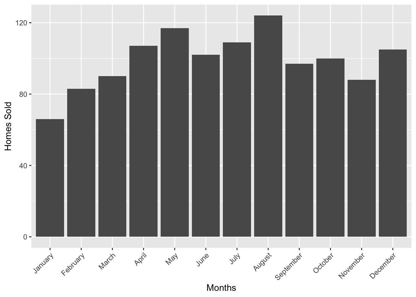
txhousing contains monthly data about home purchases, listings, median home cost, etc. If you’d like to visualize certain metrics by city, it would be trivial to do so in R. Let’s take a look at the number of home sales each month in San Angelo Texas (where i coincidentally grew up) for the year 2002.

txhousing %>% filter(year == 2002 & city == "San Angelo") %>% ggplot(aes(x = monthname, y = sales)) + geom_col() + theme(axis.text.x = element_text(angle = 45, hjust = 1))+ xlab("Months") + ylab("Homes Sold")

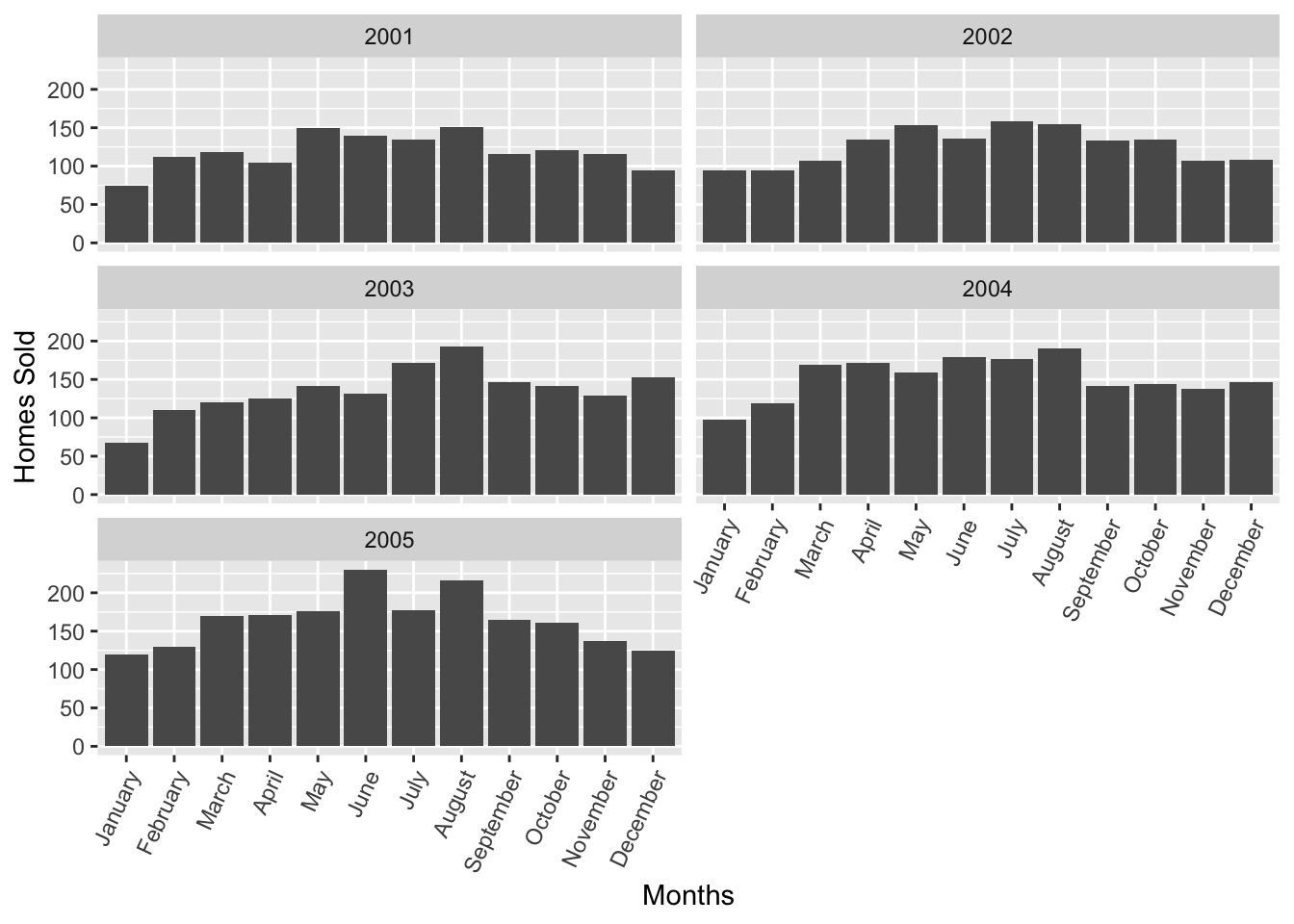
Great, this looks like your standard column graph! What if we were tasked to do it for Abilene next, and not only for the year 2002, but for the range of 2001-2005, faceted by year. Well, such a request wouldn’t be that difficult, we can just grab the previous chunk of code and make some modifications.

txhousing %>% filter(year %in% c(2001,2002,2003,2004,2005) & city == "Abilene") %>% ggplot(aes(x = monthname, y = sales)) + geom_col() + facet_wrap(~year,ncol = 2) + theme(axis.text.x = element_text(angle = 65, hjust = 1)) + xlab("Months") + ylab("Homes Sold")

Both of these plots look great, but it’s not difficult to imagine a scenario where we’re asked for more sales data from other towns nearby, or on the other side of Texas. Instead of repeatedly copying and pasting the same chunks, and modifying the relevant bits, we can construct a really simple function on the fly.

PlotHomeSales <- function(citystr,years, df){
  df %>% filter(city == citystr & year %in% years) %>% ggplot(aes(x = monthname, y = sales)) + geom_col() + facet_wrap(~year,ncol = 2)  + theme(axis.text.x = element_text(angle = 45, hjust = 1)) + xlab("Months") + ylab("Homes Sold")
}

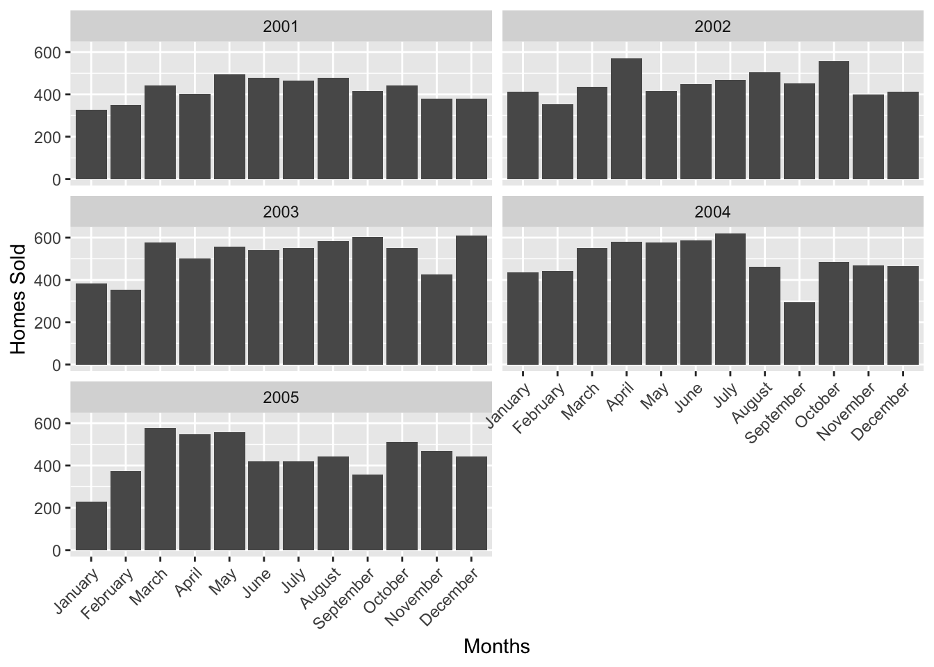
Let’s go ahead and call our function for El Paso, through the years 2001-2002.

salesyears <- seq(2001,2005, by = 1)
PlotHomeSales("El Paso", salesyears, txhousing)

As you can see, this greatly simplifies repetitive tasks. We can continue on further, and build onto our function. Our dataframe txhousing has 10 columns, three of which are the year, month (numerical) and month name.

txhousing %>% head(20)

## # A tibble: 20 x 10
##    city   year month sales volume median listings inventory  date monthname
##    <chr> <int> <int> <dbl>  <dbl>  <dbl>    <dbl>     <dbl> <dbl> <fct>    
##  1 Abil…  2000     1    72 5.38e6  71400      701       6.3 2000  January  
##  2 Abil…  2000     2    98 6.50e6  58700      746       6.6 2000. February 
##  3 Abil…  2000     3   130 9.28e6  58100      784       6.8 2000. March    
##  4 Abil…  2000     4    98 9.73e6  68600      785       6.9 2000. April    
##  5 Abil…  2000     5   141 1.06e7  67300      794       6.8 2000. May      
##  6 Abil…  2000     6   156 1.39e7  66900      780       6.6 2000. June     
##  7 Abil…  2000     7   152 1.26e7  73500      742       6.2 2000. July     
##  8 Abil…  2000     8   131 1.07e7  75000      765       6.4 2001. August   
##  9 Abil…  2000     9   104 7.62e6  64500      771       6.5 2001. September
## 10 Abil…  2000    10   101 7.04e6  59300      764       6.6 2001. October  
## 11 Abil…  2000    11   100 7.89e6  70900      721       6.2 2001. November 
## 12 Abil…  2000    12    92 7.28e6  65000      658       5.7 2001. December 
## 13 Abil…  2001     1    75 5.73e6  64500      779       6.8 2001  January  
## 14 Abil…  2001     2   112 8.67e6  68900      700       6   2001. February 
## 15 Abil…  2001     3   118 9.55e6  72300      738       6.4 2001. March    
## 16 Abil…  2001     4   105 8.70e6  71500      810       7   2001. April    
## 17 Abil…  2001     5   150 1.18e7  71000      772       6.6 2001. May      
## 18 Abil…  2001     6   139 1.13e7  78100      825       7.2 2001. June     
## 19 Abil…  2001     7   134 1.32e7  86700      801       7.1 2002. July     
## 20 Abil…  2001     8   151 1.18e7  69000      891       7.7 2002. August

Let’s say we happen to have dataframes from multiple states with the same structure, and we’d like to be able to build a function that is not limited to returning a column plot of the sales per month. We’d like to be able to supply an argument to our function that dictates what we’d like to visualize, so that we’re able to visualize sales, volume, median, or listings on a whim.

PlotHomeSales <- function(citystr,years, colname, df){
txhousing %>%  filter(city == citystr & year %in% years) %>% select(year, monthname, selected = contains(colname))%>% ggplot(aes(x = monthname, y = selected)) + geom_col() + facet_wrap(~year,ncol = 2)  + theme(axis.text.x = element_text(angle = 45, hjust = 1)) + xlab("Months") + ylab(colname)
}

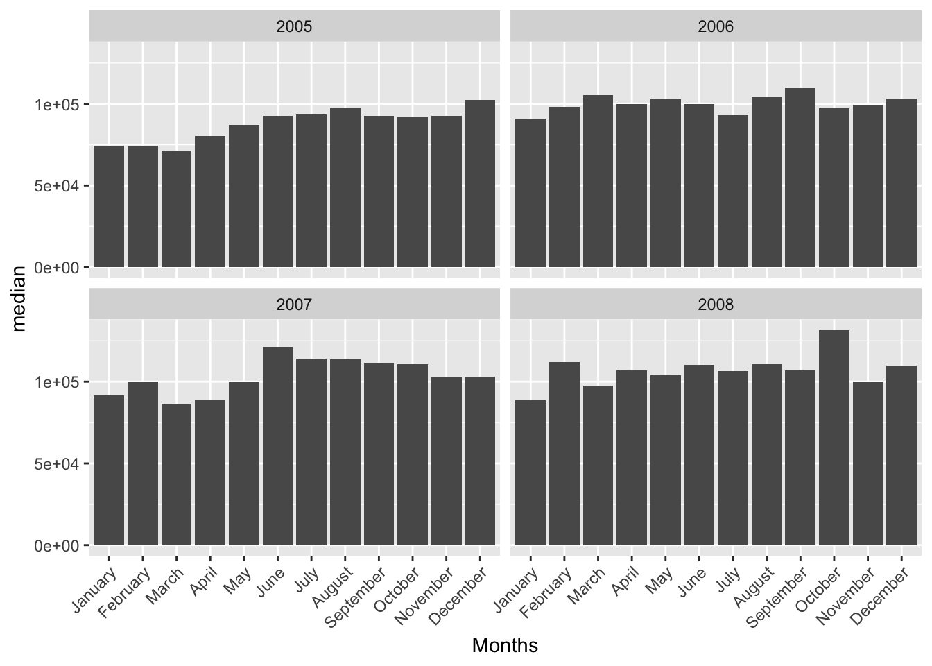
We can go ahead and visualize the median sale price of home sales each month through 2005-2008 for Abilene.

PlotHomeSales("Abilene", c(2005,2006,2007,2008), "median", txhousing)

Let’s move away from visualization, and write a function for imputing missing values, a process that’s heavily relied on in data analytics. Data imputation functions already exist. In fact, there’s an entire package dedicated to imputation called MICE (Multivariate Imputation Via Chained Equations), but we will go ahead an construct a rudimentary function just to illustrate the usefulness of function writing.

First, let’s heed a word of caution: The type of imputation we’ll be doing is extremely simple, therefore it is not the most advanced or precise method for training ML models, or for exhaustive analysis.

The two most fundamental imputation methods are median, and mean. Furthermore, two seperate types exist Generalized Imputation, and Similar Case Imputation. Generalized imputation applies an imputation method to a column irregardless of values in other columns. Similar Case Imputation takes other columns into account. Let’s look at a quick example, a dataframe that describes the age and height of differing genders.

GenderAttrib

##       gen height age
## 1  Female   2.18  NA
## 2  Female   1.83  19
## 3  Female     NA  20
## 4  Female     NA  NA
## 5  Female   2.26  19
## 6    Male   1.84  29
## 7    Male     NA  29
## 8    Male     NA  30
## 9    Male   1.97  NA
## 10   Male   1.91  30

We can go ahead and write a quick function that applies a general imputation method of either mean, or median. Our function will take a dataframe, column name, and method argument (mean or median), and return a vector with values imputed using the generalized imputation type. We can go ahead and replace the old column with the new using the extraction operator $.

imputevalues <- function(dfimpute, columnname, method = "mean"){
  if(method == "mean"){
  meanval <- dfimpute %>% select(contains(columnname)) %>% sapply(mean, na.rm = TRUE)
  
  dfimpute[is.na(dfimpute[,c(columnname)]),c(columnname)] <- meanval
  
  return(dfimpute[,c(columnname)] )
  }
  if(method == "median"){
  meanval <- dfimpute %>% select(contains(columnname)) %>% sapply(median, na.rm = TRUE)
  dfimpute[is.na(dfimpute[,c(columnname)]),c(columnname)] <- meanval
  return(dfimpute[,c(columnname)])
  } 
  else return(stop('Unknown method...'))
}

Let’s call it on our dataset:

imputevalues(GenderAttrib, "height")

##  [1] 2.180000 1.830000 1.998333 1.998333 2.260000 1.840000 1.998333
##  [8] 1.998333 1.970000 1.910000

Let’s call it using the median function for age

imputevalues(GenderAttrib, "age", "median")

##  [1] 29 19 20 29 19 29 29 30 29 30

Wrap-up

I hope this article has piqued your interest in programming with R. While most of the aspects of function writing covered herein have been at a high level, there are a vast number of resources online that delve deeper into this topic.

J Caro's Blog