Hotel Cancellations: A Business Application of Machine Learning
Introduction
It’s late April, and COVID19 has rattled economies across the world. Even worse, it’s caused a catastrophic number of deaths in countries that were under-prepared, causing shortages in PPE and prophylactics. Some businesses in industries that depend on travel are folding, consequently laying off employees and personnel across organizations.
This article doesn’t attempt to address the strain hotels face when it comes to dealing with COVID19. It can however, increase the revenue of hotels throughout the year without any capital investment! This draws off a very polarizing practice employed by airlines: overbooking. Overbooking occurs when airlines book more seats than exist on a given flight. They’re not stupid, they know exactly how many seats there are on each flight. They just attempt to overbook the exact quantity of seats that they expect to be cancelled, to maximize their profit. Without overbooking the airlines miss out on expected, or additional revenue from those cancelled seats. It depends on the refundability of the tickets. If a ticket for a given seat is refundable, the airline loses out on the revenue of that seat. If the ticket is not refundable, the airline can effectively increase their revenue by collecting the cancellation fee and the additional revenue of getting a new passenger in that seat.
This translates perfectly well with Hotels.
Objective
In this article, we hope to outline a method that identifies notable characteristics of hotel reservations resulting in cancellations, or check-ins. After performing some PCA, we’ll go ahead and utilize a few ML algorithms and assess their performance. We’ll follow this set of procedures:
- Summarizing our data set, and conducting any cleaning or pre-processing if necessary
- Conducting some exploratory data analysis to identify any useful explanatory variables.
- Carry out some one-hot variable encoding (as needed) to obtain a dataset with a uniform set of classes.
- We’ll conduct some Principle Component Analysis with the goal of reducing dimensionality and increasing variance.
- Finally, we’ll go ahead and train a few machine learning models with different types of algorithms. We’ll evaluate their performance with ROC curves, confusion matrices, and evaluation metrics (sensitivity, specificity, etc.).
Let’s get started!
Data Set
The variables of our dataset are displayed below. The response variable of interest is is_canceled, which has been encoded to a bi-level factor. Some of the explanatory variables contain straightforward names, such as arrival_date, stays_in_weekend_nights, etc. Some are labeled, and encoded in an un-intuitive manner to protect specific business practices, like agent, company, etc.
At first glance, we can expect that some of these explanatory variables will have a strong effect on the response variable. Namely, the quantity of adults, previous_cancellations, and previous_bookings_not_cancelled, but we’ll examine these further in the exploratory data analysis section. Other variables like reservation_status_date, and reservation_status are not pertinent to the scope of this ML modeling. We’ll remove these variables from out dataset.
Hotel.Data %>% str()
## 'data.frame':    119390 obs. of  32 variables:
##  $ hotel                         : Factor w/ 2 levels "City Hotel","Resort Hotel": 2 2 2 2 2 2 2 2 2 2 ...
##  $ is_canceled                   : int  0 0 0 0 0 0 0 0 1 1 ...
##  $ lead_time                     : int  342 737 7 13 14 14 0 9 85 75 ...
##  $ arrival_date_year             : int  2015 2015 2015 2015 2015 2015 2015 2015 2015 2015 ...
##  $ arrival_date_month            : Factor w/ 12 levels "January","February",..: 6 6 6 6 6 6 6 6 6 6 ...
##  $ arrival_date_week_number      : int  27 27 27 27 27 27 27 27 27 27 ...
##  $ arrival_date_day_of_month     : int  1 1 1 1 1 1 1 1 1 1 ...
##  $ stays_in_weekend_nights       : int  0 0 0 0 0 0 0 0 0 0 ...
##  $ stays_in_week_nights          : int  0 0 1 1 2 2 2 2 3 3 ...
##  $ adults                        : int  2 2 1 1 2 2 2 2 2 2 ...
##  $ children                      : int  0 0 0 0 0 0 0 0 0 0 ...
##  $ babies                        : int  0 0 0 0 0 0 0 0 0 0 ...
##  $ meal                          : Factor w/ 5 levels "BB","FB","HB",..: 1 1 1 1 1 1 1 2 1 3 ...
##  $ country                       : Factor w/ 178 levels "ABW","AGO","AIA",..: 137 137 60 60 60 60 137 137 137 137 ...
##  $ market_segment                : Factor w/ 8 levels "Aviation","Complementary",..: 4 4 4 3 7 7 4 4 7 6 ...
##  $ distribution_channel          : Factor w/ 5 levels "Corporate","Direct",..: 2 2 2 1 4 4 2 2 4 4 ...
##  $ is_repeated_guest             : int  0 0 0 0 0 0 0 0 0 0 ...
##  $ previous_cancellations        : int  0 0 0 0 0 0 0 0 0 0 ...
##  $ previous_bookings_not_canceled: int  0 0 0 0 0 0 0 0 0 0 ...
##  $ reserved_room_type            : Factor w/ 10 levels "A","B","C","D",..: 3 3 1 1 1 1 3 3 1 4 ...
##  $ assigned_room_type            : Factor w/ 12 levels "A","B","C","D",..: 3 3 3 1 1 1 3 3 1 4 ...
##  $ booking_changes               : int  3 4 0 0 0 0 0 0 0 0 ...
##  $ deposit_type                  : Factor w/ 3 levels "No Deposit","Non Refund",..: 1 1 1 1 1 1 1 1 1 1 ...
##  $ agent                         : Factor w/ 334 levels "1","10","103",..: 334 334 334 157 103 103 334 156 103 40 ...
##  $ company                       : Factor w/ 353 levels "10","100","101",..: 353 353 353 353 353 353 353 353 353 353 ...
##  $ days_in_waiting_list          : int  0 0 0 0 0 0 0 0 0 0 ...
##  $ customer_type                 : Factor w/ 4 levels "Contract","Group",..: 3 3 3 3 3 3 3 3 3 3 ...
##  $ adr                           : num  0 0 75 75 98 ...
##  $ required_car_parking_spaces   : int  0 0 0 0 0 0 0 0 0 0 ...
##  $ total_of_special_requests     : int  0 0 0 0 1 1 0 1 1 0 ...
##  $ reservation_status            : Factor w/ 3 levels "Canceled","Check-Out",..: 2 2 2 2 2 2 2 2 1 1 ...
##  $ reservation_status_date       : Factor w/ 926 levels "2014-10-17","2014-11-18",..: 122 122 123 123 124 124 124 124 73 62 ...
Hotel.Data %<>% select(-c("reservation_status", "reservation_status_date"))First, we should identify any missing observations in our data set. We can use gg_miss_var from the package naniar.
### From package naniar
gg_miss_var(Hotel.Data)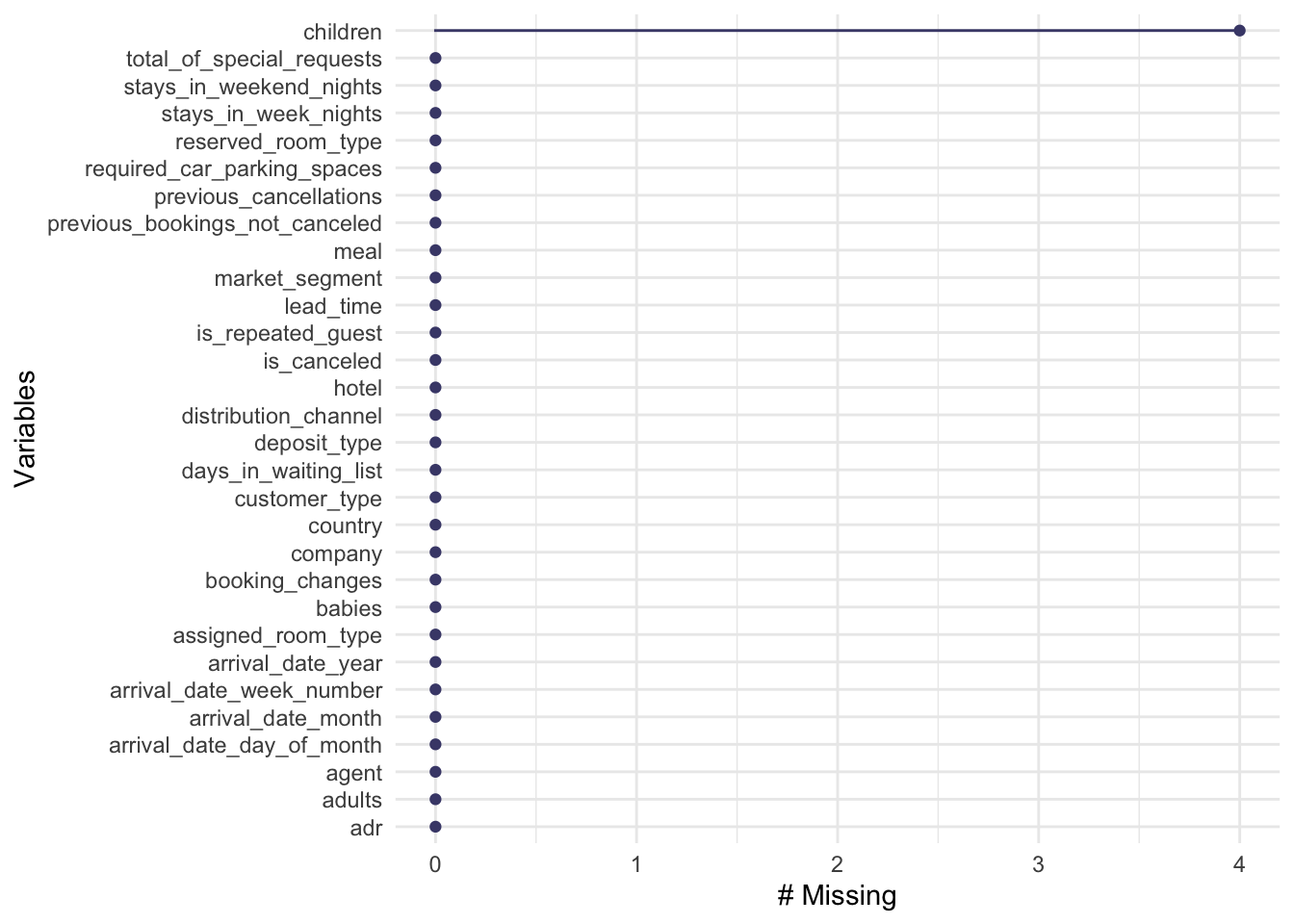
Awesome. We have a very complete data set, which reduces work in imputation. Let’s take a look at the distribution of children.
##
##      0      1      2      3     10
## 110796   4861   3652     76      1
Hotel.Data %>% mutate(is_canceled = as.factor(is_canceled)) %>% filter(!is.na(children)) %>% ggplot(aes(x = children, fill = is_canceled)) + geom_histogram(binwidth = 1) + scale_y_log10() + ggtitle("Number Of Reservations By Quantity Of Children (Scaled)")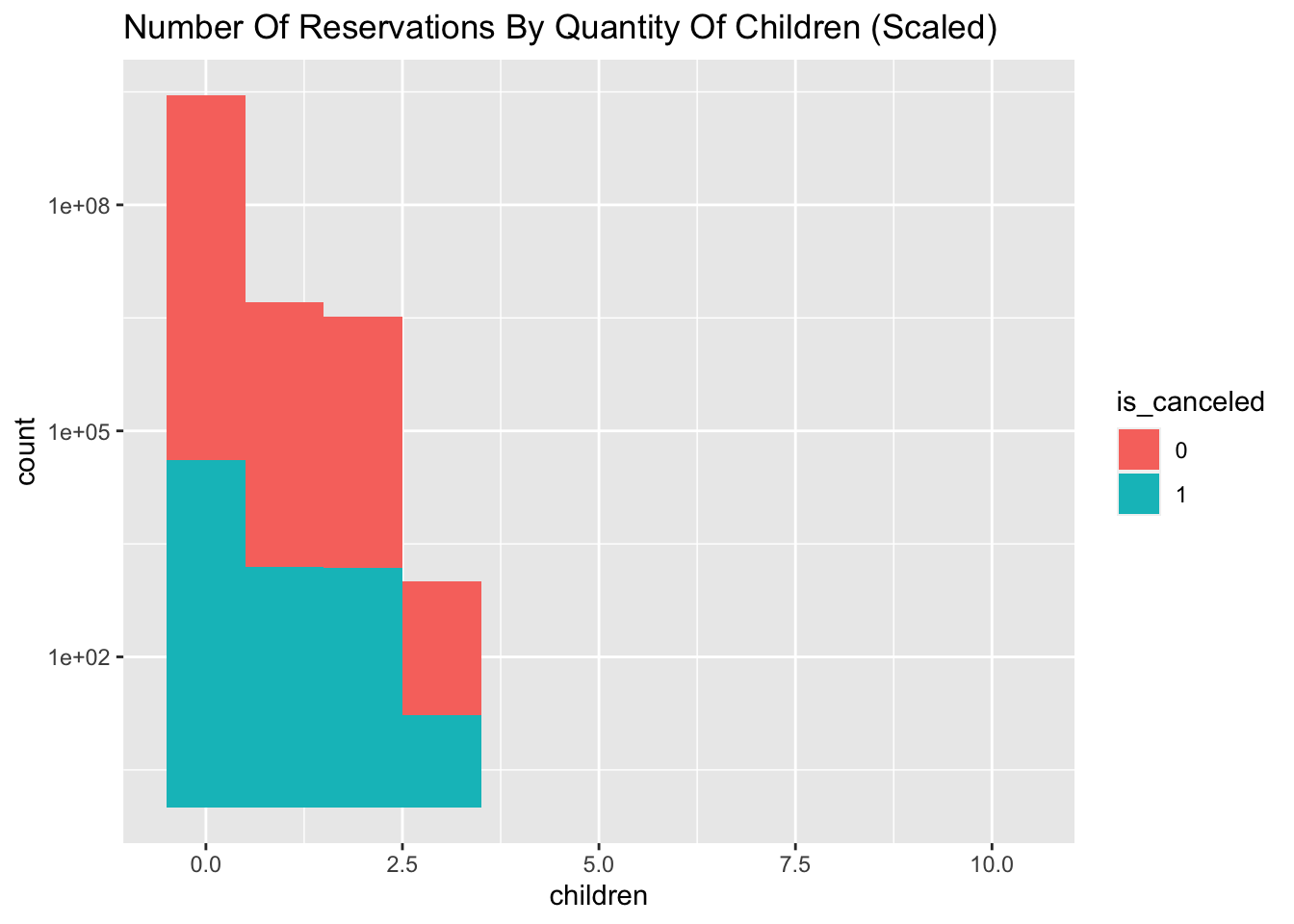
With such a large proportion of our dataset containing zero children, it would be appropriate to perform a median imputation.
Hotel.Data$children[is.na(Hotel.Data$children)] <- median(Hotel.Data$children, na.rm = TRUE)Before we get delve into any sort of analysis, we should determine what proportion of our dataset is made up of cancelled reservations.
Hotel.Data %>% mutate(is_canceled = as.factor(is_canceled))%>% group_by(is_canceled) %>% summarize(Reservations = n()) %>% ungroup() %>% mutate(Total = sum(Reservations), Proportion = paste0(round(Reservations/Total,4)*100, "%")) %>% ggplot(aes(x = is_canceled, y = Reservations, fill = is_canceled)) + geom_col() + geom_label(aes(label = Proportion))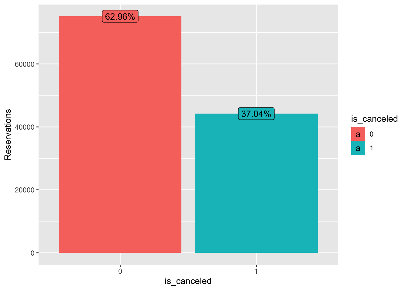
So our data is slightly imbalanced. Luckily for us, we can address this when we create our k-fold cross validation splits.
Exploratory Data Analysis & Visualizations (EDA)
Now that we’re certain we have a clean and complete set of data, we can turn our attention towards explanatory variables of interest. Referencing the output of str() above, we can identify several variables that might have an effect on reservation cancellations. The first metric of interest is lead_time, which is the quantity of days the reservation was made in anticipation to check-in.
Hotel.Data %>%mutate(is_canceled = as.factor(is_canceled)) %>% ggplot(aes(x = is_canceled, y = lead_time)) + geom_violin() + ggtitle("Lead-time vs Reservation Status")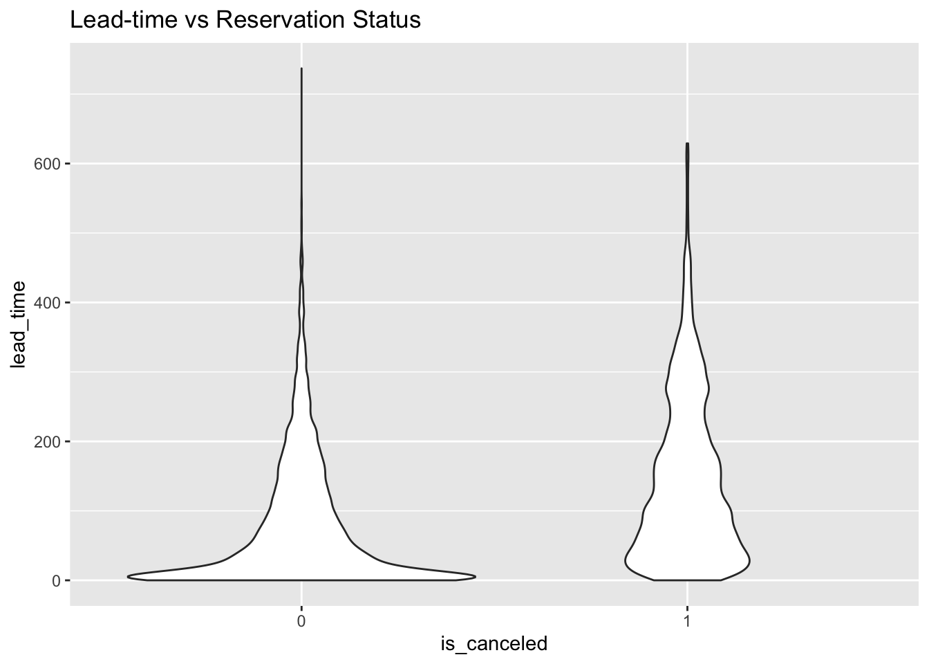
This violin plot illustrates that a larger portion of cancelled reservations were made farther in anticipation, compared to reservations that successfully resulted in guest check-ins. Another variable of interest is deposit_type, which illustrates the deposit refundability for a particular reservation. The three types are No Deposit, where no deposit is required to make a reservation. The other two are Non Refundable and Refundable. Usually hotel reservations with Non Refundable reservations are relatively cheaper than the other deposit types. We’ll go ahead and get a tally of each deposit policy in our dataset.
DepositTypeCount <- Hotel.Data %>% group_by(deposit_type) %>% summarize(Reservation_Count = n())
DepositTypeCount
## # A tibble: 3 x 2
## deposit_type Reservation_Count
## <fct> <int>
## 1 No Deposit 104641
## 2 Non Refund 14587
## 3 Refundable 162We see that a significant majority of our dataset contains reservations that required no deposit, with a miniscule amount containing refundable reservations.
Hotel.Data %>% mutate(is_canceled = as.factor(is_canceled)) %>% ggplot(aes(x = deposit_type, fill = is_canceled)) + geom_bar(position = "fill") + ylab("Proportion") + xlab("Deposit Type")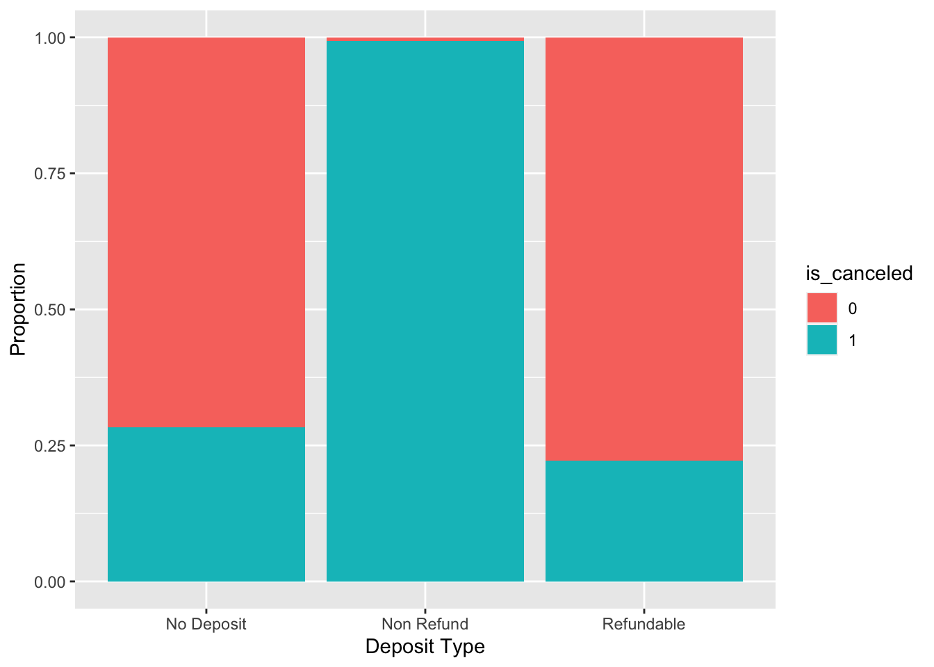
Apart from the imbalance, it seems that an overwhelming amount of non-refundable reservations ended up in cancellations. We can shift our attention towards the previous quantity of reservations that resulted in cancellations or check ins, made by the individual booking the reservations.
Hotel.Data %>% mutate(is_canceled = as.factor(is_canceled)) %>% select(is_canceled, previous_cancellations, previous_bookings_not_canceled) %>% mutate(propnoncancelled = if_else(is.na(previous_bookings_not_canceled / (previous_cancellations + previous_bookings_not_canceled)), 0, (previous_bookings_not_canceled / (previous_cancellations + previous_bookings_not_canceled )))) %>% gather(key = "Metric", value = "Quantity", 2:4) %>% ggplot(aes(x = Quantity, fill = is_canceled)) + geom_histogram(bins = 12) + facet_wrap(~Metric, scales = "free_x", ncol = 1) + scale_y_log10() 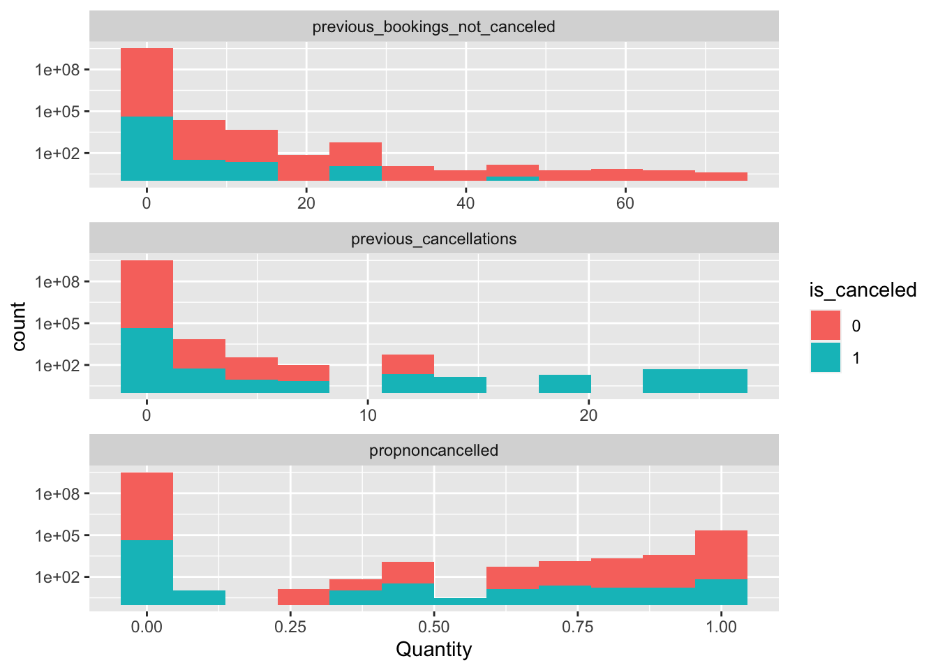
The results are what we’d expect. Bookings made by individuals with a high amount of cancellations resulted in more cancellations. Conversely, bookings made by individuals with a high number of non-cancellations, resulted in less cancellations. I have also included a transformation of the two variables as noted in the code snippet, that will be used later on. Let’s take a look at the proportion of cancellations throughout the year, grouped together by months.
Hotel.Data %>% ggplot(aes(x = arrival_date_month, fill = as.factor(is_canceled))) + geom_bar(position = "fill") + theme(axis.text.x = element_text(angle = 40, hjust = 1)) + ylab("proportion")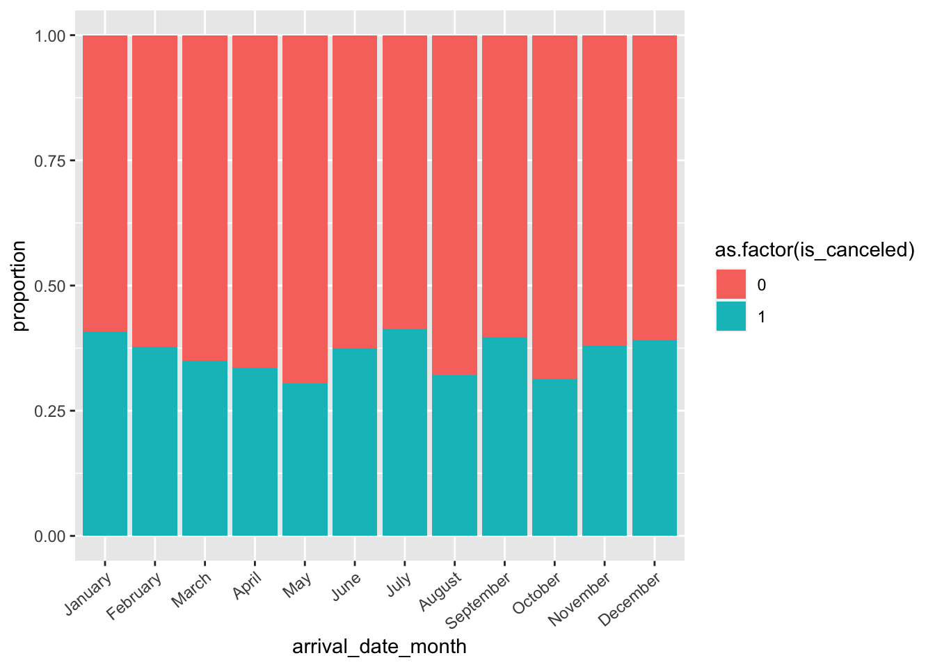
There seems to be an increase in cancellations on the tail ends of the year, as well as a breif spike in the summer months. Lastly, we’ll take a look at the proportion of cancellations by continent. This explanatory variable is obtained by utilizing the country code function, and the country variable. Since our dataset contains a large amount of countries, it’s cumbersome to visualize and may provide little value since some countries could be under-represented. Furthermore, a lot of machine learning algorithms have factor limitations which are surpassed by the number of countries contained in this dataset (178 countries, as seen in str(Hotel.Data))
Hotel.Data$continent <- Hotel.Data$country %>% countrycode(origin = "iso3c",destination = "continent")
Hotel.Data$continent[is.na(Hotel.Data$continent)]<- "Other"
Hotel.Data$continent %<>% as.factor()
Hotel.Data %>% mutate(is_canceled = as.factor(is_canceled)) %>%  ggplot(aes(x = continent, fill = is_canceled)) + geom_bar(position = "fill")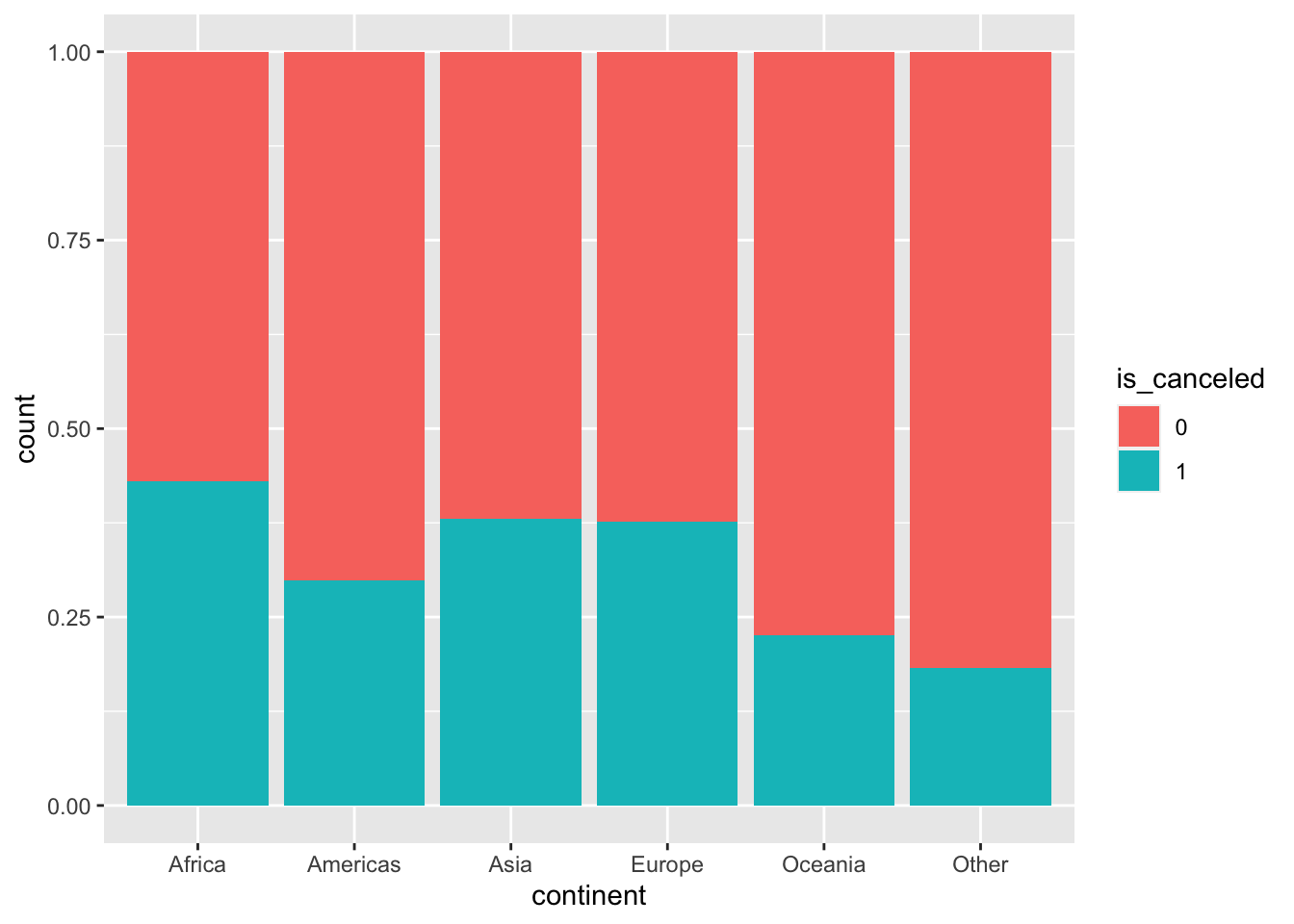
It seems like reservations made by individuals in Africa have a high cancellation rate, followed closely by a tie between Asia and Europe.
Now that we’ve looked at the structure of our data, and done some exploratory data analysis, we can move onto variable encoding.
Variable Encoding
Since we’re going to be performing principle component analysis (PCA) on our dataset, we have to make sure our dataset is of a uniform numeric class throughout our variables. We can obtain all of the original numeric variables by using select_if.
Hotel.Data.Numeric <- Hotel.Data %>% select_if(is.numeric)
Hotel.Data.Numeric %>% dim()
## [1] 119390 18Uh-oh! We have reduced the number of explanatory variables in our dataset from 31 to 18. We’re effectively throwing out 13 explanatory variables that could potentially posses valuable information. We can address this by performing one-hot encoding on our factor variables. It’s worth noting that we can’t do this indiscriminately, as we’d run the risk of significaly increasing the dimensionality of our dataset and running into memory or performance issues later on.
When we encode an n-level factor variable utilizing the one-hot encoding method, we effectively create n variables (or (n-1) depending on the method). So, if we have p factor variables each with n1, n2, n3, n4 …nn levels we’ll find that we effectively create up to n1 + n2 + n3 +… nn variables. Unfortunately, most of these rows will be sparse, because one hot encoding encodes a level of a factor into a binary variable. Why is this en issue? Well, we end up utilizing a lot of memory storing 0 values on those rows. It may not be troubling when dealing with small to moderately sized datasets, but could cause issues when working with very large and wide datasets. Lets look at a sample dataframe where we have a row that contains two variables: day of the week, and a color.
#Declaring some sample arrays and declaring a dataframe
DOW <- c("Monday", "Tuesday", "Wednesday", "Thursday", "Friday", "Saturday", "Sunday")
days_of_week <- rep(DOW, times = 2)
Color <- c("Red", "Blue")
colors <- rep(Color, times = 7)
sample_df <- data.frame(days_of_week = as.factor(days_of_week), colors = as.factor(colors))
sample_df
## days_of_week colors
## 1 Monday Red
## 2 Tuesday Blue
## 3 Wednesday Red
## 4 Thursday Blue
## 5 Friday Red
## 6 Saturday Blue
## 7 Sunday Red
## 8 Monday Blue
## 9 Tuesday Red
## 10 Wednesday Blue
## 11 Thursday Red
## 12 Friday Blue
## 13 Saturday Red
## 14 Sunday BlueHere is the dataframe after one-hot encoding both columns. Note the sparseness.
cbind(class2ind(sample_df$days_of_week), class2ind(sample_df$colors))## Friday Monday Saturday Sunday Thursday Tuesday Wednesday Blue Red
## 1 0 1 0 0 0 0 0 0 1
## 2 0 0 0 0 0 1 0 1 0
## 3 0 0 0 0 0 0 1 0 1
## 4 0 0 0 0 1 0 0 1 0
## 5 1 0 0 0 0 0 0 0 1
## 6 0 0 1 0 0 0 0 1 0
## 7 0 0 0 1 0 0 0 0 1
## 8 0 1 0 0 0 0 0 1 0
## 9 0 0 0 0 0 1 0 0 1
## 10 0 0 0 0 0 0 1 1 0
## 11 0 0 0 0 1 0 0 0 1
## 12 1 0 0 0 0 0 0 1 0
## 13 0 0 1 0 0 0 0 0 1
## 14 0 0 0 1 0 0 0 1 0Additionally, class2ind has an argument for bi-level factors that allow you to encode into a single column by encoding 1 for the first level and 0 for the second.
Now that we’re more familiar with one-hot encoding, we’ll go ahead and encode factor variables in our dataset, and add them to Hotel.Data.Numeric. We’ll keep the EDA we did earlier in mind. We’ll go ahead and exclude factor variables with a large amount of levels to avoid significantly increasing the size of our dataset.
Hotel.Data.Numeric <- cbind(Hotel.Data.Numeric, class2ind(Hotel.Data$deposit_type))Let’s take a look at the dimensions of our data set after encoding:
Hotel.Data.Numeric %>% dim()## [1] 119390 63Feature Transformation & Principle Component Analysis
Now that we have kept most of our factor variables, and have performed a one hot encoding method to keep as much as the information as possible, we see that we have introduced 32 additional columns into our dataset. This means, we have to try and address the daunting task of figuring out which variables are the most salient to our objective in predicting cancellations. We can identify pertinent variables by transforming them into new ones using Princple Component Analysis. This step has a few pros and cons:
Pros:
- Our dataset becomes leaner and we can keep most of the information.
- Depending on the model we wish to choose, PCA reduces any high correlated explanatory variables that may exist.
- All of the resulting variables (principle components) will be orthogonal and thus have zero covariance (covariance can be detrimental to certain ML algorithms).
Cons:
- We lose transparency with respect to the effect of our original variables on the resultant model.
- We introduce an additional step of encoding new data with our PCA model.
Since we have done some EDA, and we’re mostly interested in increasing the accuracy of our model we’ll procede with PCA. Calling the function, we’ll elect to scale and center. Scaling prevents any undesirable effect of mixing explanatory variables with different units (think mm, days, and years).
pca.mod <- prcomp(Hotel.Data.Numeric[,-1], scale.= TRUE)This isn’t an article about PCA You can find that here, but we’ll go ahead and plot the contribution of our original variables on our new PCA transformed variables.
fviz_pca_var(pca.mod, col.var = "contrib" ,repel = TRUE)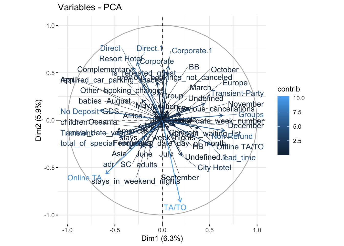
This plot illustrates the loading weights of each variable on Dim1 and Dim2. The projection of each arrow along Dim1 and Dim2 illustrates how much weight they contribute to the resultant PCA variables. Another notable feature of this visualization, is that arrows pointing in similar directions are positively correlated, while arrows in opposite directions are negatively correlated.
Let’s go ahead and look at the percentage of variance explained by each variable.
fviz_eig(pca.mod,ncp = 20)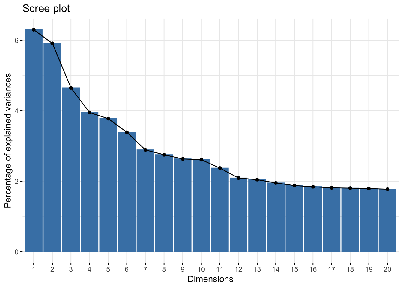
In the context of PCA, this visualization is reffered to as a “Scree Plot”. It visualizes the contribution of each dimension to the total variance of the dataset. This is where we can pick a subset of the variables to keep and utilize in our ML training and testing process. While there’s no established convention to follow when choosing the size of your subset, it’s pretty common to cut off the variables past an “elbow” in the scree plot. Here, an elbow is the point where the slope of variation with regards to dimension numbers drastically changes. We can see that we have one at 7 dimensions. There’s not much change in the contribution of variance for variables 7-10 and beyond.
In the remainder of this article I will use a subset of the first 12 variables though, seeing as the change in variance is negligible from 13 and beyond. However, if this was a more detailed article, I’d train models with both sets, and compare ROC metrics after tuning. We will omit this however, for brevity.
Training & Cross Validation
This is where we finally get to tune and train our models. Now that we have the dataset resulting from PCA, all that’s left is to join the cancellation variable for training. Also, we’ll go ahead and define the type of cross validation we’d like to perform. Since there is a considerable class imbalance in our response variable we need to address any over/under sampling that may occur when creating our cross validation folds. Luckily for us, the function createFolds from caret addresses this, and we’re able to easily create a k-fold object with balanced response variable classes across each fold.
In addition to joining the response variable, and creating our k-fold object, we’ll declare our trainControl parameter where we describe the type of summary function we’d like, and indicate that we would like the class probabilities of our response variable, verbose iterations while training, as well as saving the predictions. In the index argument, we’ll supply the k-fold cross validation object we created.
## Create Folds
Hotel.PCA<- cbind(is_canceled = as.factor(if_else(Hotel.Data$is_canceled == 1, "Cancelled", "Not_Cancelled")), as.data.frame(pca.mod$x[,1:12]))
nFolds <- createFolds(Hotel.PCA$is_canceled, k = 5)
tControl <- trainControl(
  summaryFunction = twoClassSummary,
  classProbs =  TRUE,
  verboseIter = TRUE,
  savePredictions = TRUE,
  index = nFolds
)
The Machine Learning algorithms that we’ll be using to perform predict cancellations will be the logistic general linear model, random forest, and neural net. The metric we wish to optimize is the area under our ROC curve. We can however optimize our machine learning models by tuning parameters and choosing the model that gives the best accuracy instead. For a well-rounded approach, you can use all three. In this section, we’re primarily interested in the area under the ROC curve, and the sensitivity and specificity of our resulting model.
For a more in-depth look at machine learning classifications, and definitions of relevant terms, you can find an article that I wrote last year here. This contains a more detailed process, and definitions of terms salient to assessing the effectiveness of our models.
First, we’ll start with the general linear model, or glm. There’s no tuning parameters for this model.
modelglm <- train(is_canceled ~., data = Hotel.PCA, method = "glm", trControl = tControl, metric = "ROC")## + Fold1: parameter=none
## - Fold1: parameter=none
## + Fold2: parameter=none
## - Fold2: parameter=none
## + Fold3: parameter=none
## - Fold3: parameter=none
## + Fold4: parameter=none
## - Fold4: parameter=none
## + Fold5: parameter=none
## - Fold5: parameter=none
## Aggregating results
## Fitting final model on full training setprint(modelglm)## Generalized Linear Model
##
## 119390 samples
## 12 predictor
## 2 classes: 'Cancelled', 'Not_Cancelled'
##
## No pre-processing
## Resampling: Bootstrapped (5 reps)
## Summary of sample sizes: 23877, 23878, 23878, 23878, 23879
## Resampling results:
##
## ROC Sens Spec
## 0.7923464 0.4244697 0.9601715This results in a decent ROC value, but it has low sensitivity, and high specificity. In the article I previously linked, I defined specificity and sensitivity. Sensitivity is otherwise known as the True Positive Rate, and is defined as \(TPR = \frac{TP}{TP + FN}\). Specificity is also known as the True Negative Rate and is defined as \(TNR = \frac{TN}{TN + FP}\). We can use a confusion matrix to calculate these metrics:
conf.mat <- confusionMatrix(predict(modelglm, Hotel.PCA[,-1], type = "raw"), Hotel.PCA$is_canceled)
conf.mat <- conf.mat$table
conf.mat
## Reference
## Prediction Cancelled Not_Cancelled
## Cancelled 18722 3008
## Not_Cancelled 25502 72158We can use the above table to calculate the values by hand (just to illustrate).
TPR = 18722/(18722 + 25502)
TNR = 72158/(72158 + 3008)
TPR
## [1] 0.4233448TNR## [1] 0.9599819Let’s take a look at the ROC Curve as well:
roc.glm <- roc(Hotel.PCA$is_canceled,predict(modelglm,Hotel.PCA[,-1], type = "prob")$Cancelled, direction = ">")
roc.glm <- data.frame(thresh = roc.glm$thresholds[-c(1)], sensitivity = roc.glm$sensitivities[-c(1)], specificity = roc.glm$specificities[-c(1)])
roc.glm %>% ggplot(aes(x = (1 - specificity), y = sensitivity, color = "Sensit.")) + geom_line()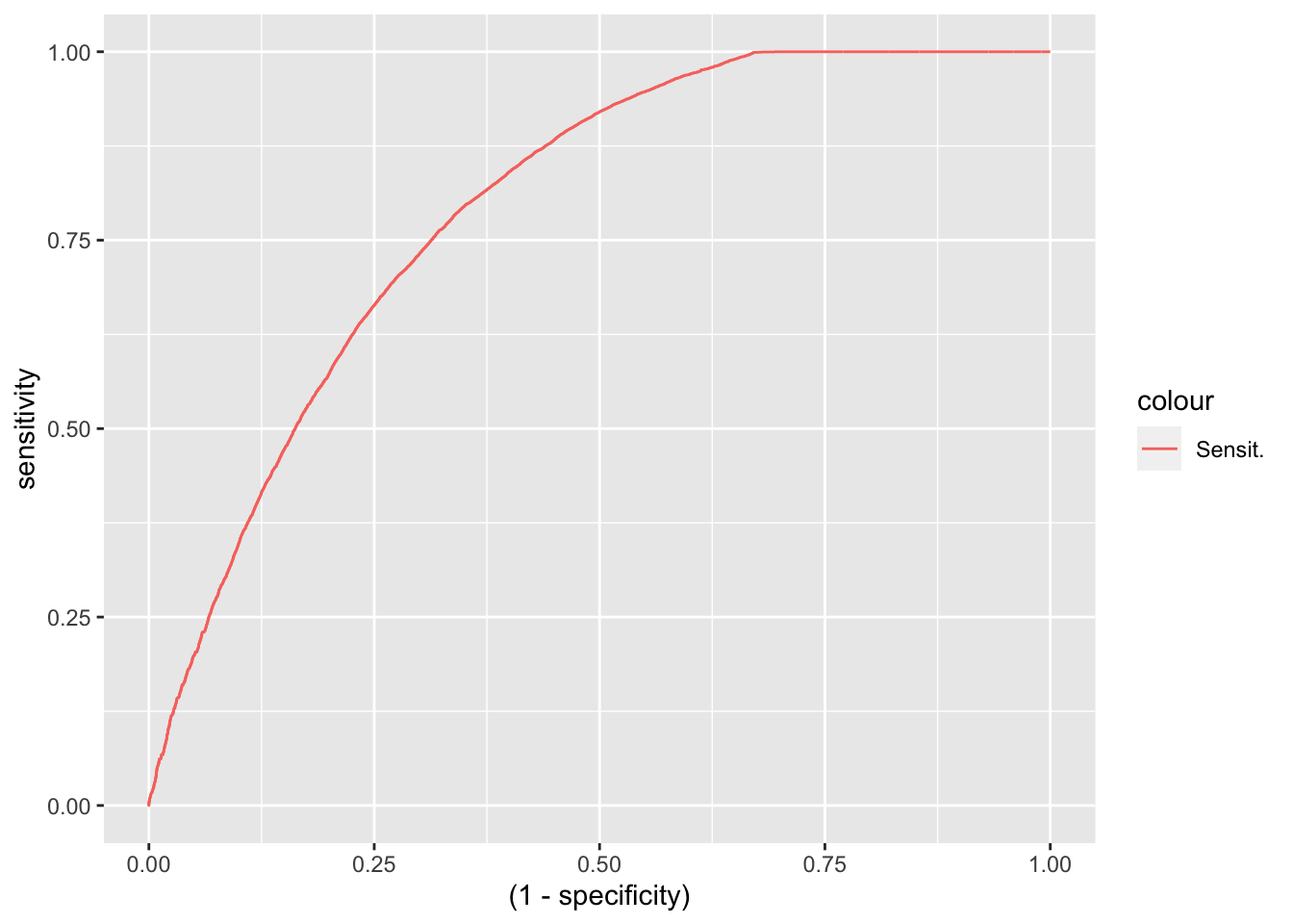
roc.models <- roc.glm
roc.models$type <- "GLM"
While the AUC (area under curve) of the ROC is a very important metric, but perhaps the most important are specificity and sensitivity. We would ideally like both high specificity and high sensitivity, but as it turns out a model with high specificity and moderate sensitivity, is more valuable than a model with moderate specificity and sensitivity. Why’s that? Let’s take a step back to how these metrics apply to our model.
In our application, a sensitivity of one means we can be very sure we’ll correctly identify every true cancellation made. Equivalently, this means that our false negatives will be zero, or that none to little of our predicted cancellations actually result in a successful check-in. Likewise, a specificity of one means that our false positives are zero. Or that none of our bookings that result in check-ins are incorrectly predicted as cancellations.
Which of these metrics can we afford to compromise? Well we can afford compromise on sensitivity, but not specificity. It’s very important we don’t misclassify check-ins as cancellations, so we should minimize false positives as much as possible. If we incorrectly classify too many actual check-ins as cancellations, we run the risk of considerable over-booking, making us liable for customers we cannot accomodate.
Let’s take a look at the two remaining models, ranger which is a random forest model, and nnet which is a neural net model. We have already tuned both of these, and the tuneGrid contains the tuning parameters with the highest AUC of the ROC.
print(rf.model)## Random Forest
##
## 119390 samples
## 12 predictor
## 2 classes: 'Cancelled', 'Not_Cancelled'
##
## No pre-processing
## Resampling: Bootstrapped (5 reps)
## Summary of sample sizes: 23877, 23878, 23878, 23878, 23879
## Resampling results:
##
## ROC Sens Spec
## 0.8831178 0.6561595 0.9218929
##
## Tuning parameter 'mtry' was held constant at a value of 5
## Tuning
## parameter 'splitrule' was held constant at a value of hellinger
##
## Tuning parameter 'min.node.size' was held constant at a value of 14roc.rf <- roc(Hotel.PCA$is_canceled,predict(rf.model,Hotel.PCA[,-1], type = "prob")$Cancelled)
roc.rf <- data.frame(thresh = roc.rf$thresholds[-c(1)], sensitivity = roc.rf$sensitivities[-c(1)], specificity = roc.rf$specificities[-c(1)])
roc.rf %>% ggplot(aes(x = (1 - specificity), y = sensitivity, color = "Sensit.")) + geom_line()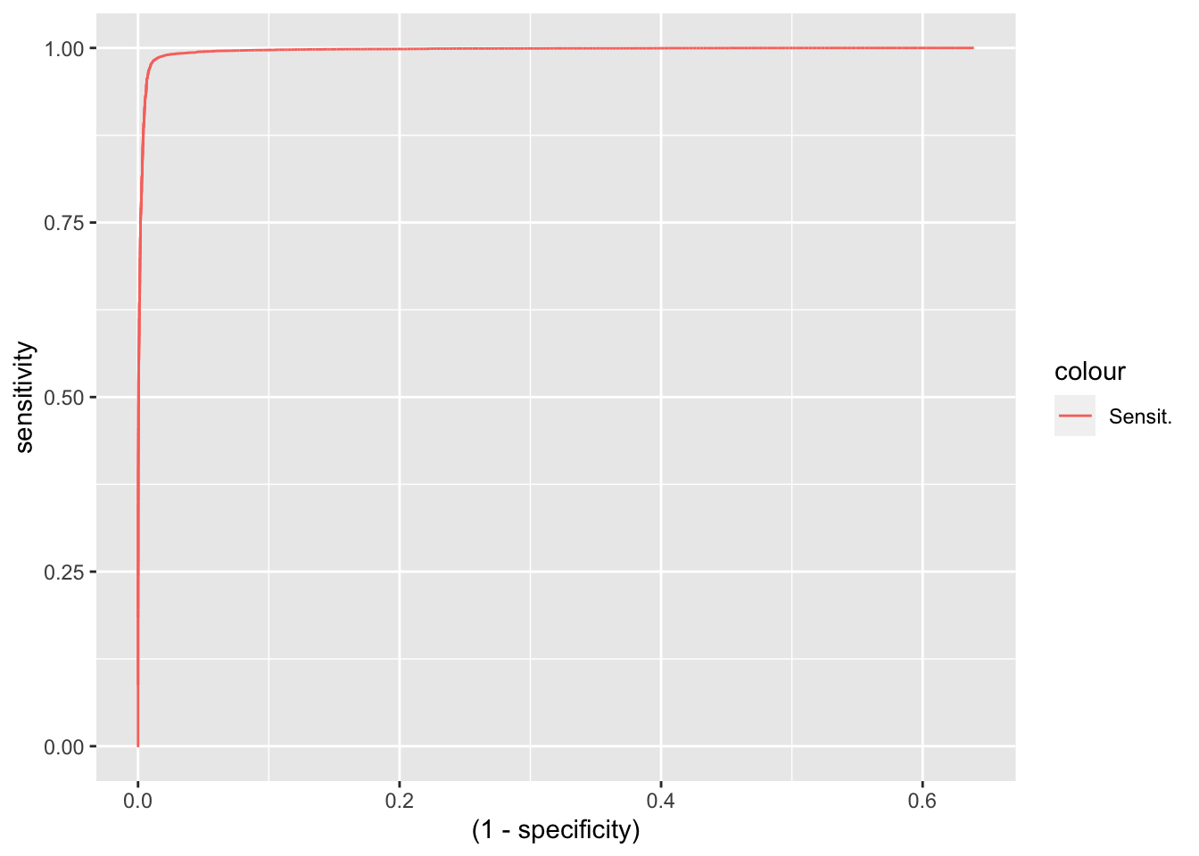
roc.rf$type <- "Random Forest"
roc.models <- rbind(roc.models, roc.rf)
conf.mat <- confusionMatrix(predict(rf.model, Hotel.PCA[,-1], type = "raw"), Hotel.PCA$is_canceled)
conf.mat <- conf.mat$table
conf.mat## Reference
## Prediction Cancelled Not_Cancelled
## Cancelled 42364 494
## Not_Cancelled 1860 74672A tuned random forest model gives us a higher specificity and sensitivity than the GLM model. Furthermore, the AUC metric is remarkably better than the GLM model. One caveat of using this model, is the length of time it takes to train.
Let’s move on to the neural net model.
net.tGrid <- expand.grid(.decay = c(0.6), .size = c(10))
nnet.model <- train(is_canceled ~ ., data = Hotel.PCA, method = "nnet",tuneGrid = net.tGrid ,trControl = tControl, maxit = 100, metric = "ROC", verbose = FALSE)print(nnet.model)## Neural Network
##
## 119390 samples
## 12 predictor
## 2 classes: 'Cancelled', 'Not_Cancelled'
##
## No pre-processing
## Resampling: Bootstrapped (5 reps)
## Summary of sample sizes: 23877, 23878, 23878, 23878, 23879
## Resampling results:
##
## ROC Sens Spec
## 0.8355331 0.5637154 0.9216401
##
## Tuning parameter 'size' was held constant at a value of 10
## Tuning
## parameter 'decay' was held constant at a value of 0.6roc.nnet <- roc(Hotel.PCA$is_canceled,predict(nnet.model,Hotel.PCA[,-1], type = "prob")$Cancelled, direction = ">")
roc.nnet <- data.frame(thresh = roc.nnet$thresholds[-c(1)], sensitivity = roc.nnet$sensitivities[-c(1)], specificity = roc.nnet$specificities[-c(1)])
roc.nnet %>% ggplot(aes(x = (1 - specificity), y = sensitivity, color = "Sensit.")) + geom_line()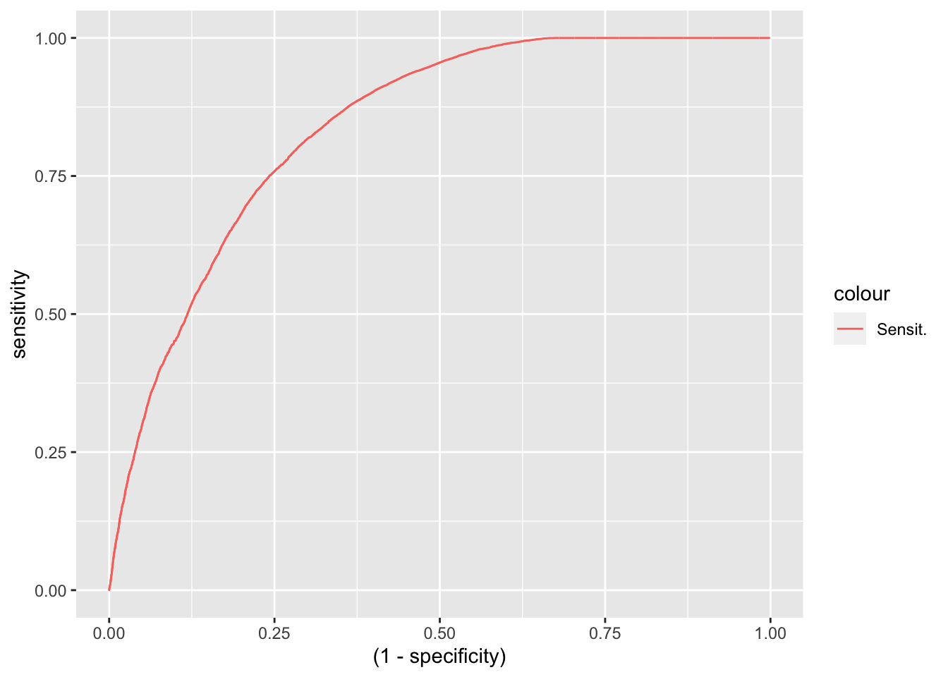
roc.nnet$type <- "Neural Net"
roc.models <- rbind(roc.models, roc.nnet)
conf.mat <- confusionMatrix(predict(nnet.model, Hotel.PCA[,-1], type = "raw"), Hotel.PCA$is_canceled)
conf.mat <- conf.mat$table
conf.mat## Reference
## Prediction Cancelled Not_Cancelled
## Cancelled 24646 5343
## Not_Cancelled 19578 69823This model is better than the GLM, but still nowhere near as good as the random forest model. The specificity of the random forest model is outstanding.
Let’s go ahead and visualize the ROC curves of all three models, color coding each.
roc.models %>% ggplot(aes(x = 1 - specificity, y = sensitivity, color = type)) + geom_line()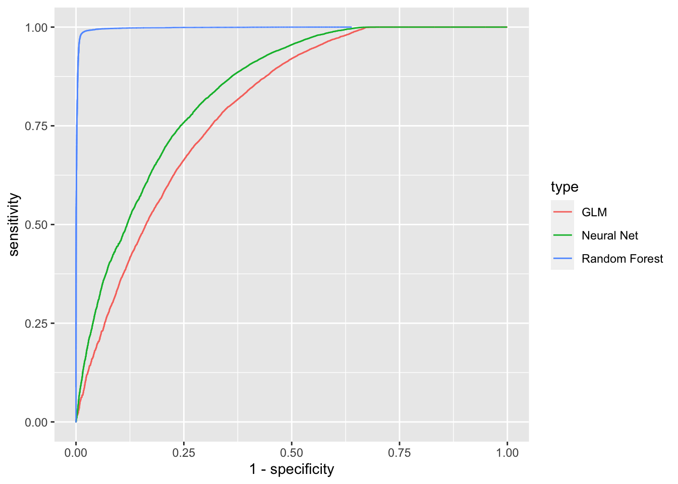
Conclusion
In this article, we have outlined a method hotels could take to predict the number of reservations they can expect result in cancellations. We did this by doing some elementary imputation, exploratory data analysis, some encoding, and ultimately trained several machine learning models. We found that our model utilizing the random forest algorithm was the most accurate, and had a much higher sensitivity, and moderately higher specificity than the GLM and Nnet models.
We could expand this article further by detailing a process hotels could use to determine the margin of their accomodations to overbook. This process would have to take the threshold of the specificity into account (false positives), as well as sensitivity. While determining the quantity of accomodations to over-book, it would be important to try and leave enough vacancies to cover the error in false positives, so that no guests are left without accomodations.